- New to JMP? Let the Data Analysis Director guide you through selecting an analysis task, an analysis goal, and a data type. Available now in the JMP Marketplace!
- See how to install JMP Marketplace extensions to customize and enhance JMP.
- Subscribe to RSS Feed
- Mark Topic as New
- Mark Topic as Read
- Float this Topic for Current User
- Bookmark
- Subscribe
- Mute
- Printer Friendly Page
Discussions
Solve problems, and share tips and tricks with other JMP users.- JMP User Community
- :
- Discussions
- :
- Re: is there a way to find the area common to two different normal distribution ...
- Mark as New
- Bookmark
- Subscribe
- Mute
- Subscribe to RSS Feed
- Get Direct Link
- Report Inappropriate Content
is there a way to find the area common to two different normal distribution curve using JMP?
I am trying to find the area under the common portion of two different normal distribution curve. How can I do that using JMP? Any simple way to do so?
- Mark as New
- Bookmark
- Subscribe
- Mute
- Subscribe to RSS Feed
- Get Direct Link
- Report Inappropriate Content
Re: is there a way to find the area common to two different normal distribution curve using JMP?
In JMP 12 there is an quite efficient Integrate() function that can be used for calculating the area confined by the minimum of the two curves.
The example below is not very useful (you'd probably want to get the parameters from the distribution platform) but may give you some ideas...
Names Default To Here(1);
// Define curves and calculate overlap area
N1 = Expr(Normal Density(x, 1, 2));
N2 = Expr(Normal Density(x, 0, 1));
ovl = Integrate(Min(N1, N2), x, ., .);
Show(ovl);


//––––––––––
// Illustration
ym = xm = (-500 :: 500) / 100;
For(i = 1, i <= N Col(xm), i++,
    ym[i] = Min(Normal Density(xm[i], 1, 2), Normal Density(xm[i], 0, 1))
);
New Window("Overlap Coefficient",
    y = Graph Box(
        Y Scale(0, 1),
        X Scale(-5, 5),
        Y Function(N1, x);
        Y Function(N2, x);
        Text({0, 0.6}, "OVL = ", ovl);
        Fill Color(1);
        Polygon(xm, ym);
    )
);
- Mark as New
- Bookmark
- Subscribe
- Mute
- Subscribe to RSS Feed
- Get Direct Link
- Report Inappropriate Content
Re: is there a way to find the area common to two different normal distribution curve using JMP?
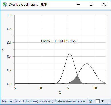
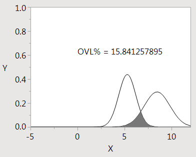
@ms Thanks for sharing this! I checked this script against an example given on the following website thanks to a colleague of mine: https://stats.stackexchange.com/questions/103800/calculate-probability-area-under-the-overlapping-ar...
With the mean and sigma parameters for the first and second distributions respectively:
"For your example, with μ1=5.28,μ2=8.45,σ1=0.91,σ2=1.36μ1=5.28,μ2=8.45,σ1=0.91,σ2=1.36, this yields: c=6.70458...c=6.70458..., and the area of the green section is: 0.158413"
The .JSL script gives the exact same result for the area of the overlapped section!
Names Default To Here(1);

// Define curves and calculate overlap area

mean1 =  5.28;
stdev1 = 0.91;

mean2  = 8.45;
stdev2 = 1.36;

N1 = Expr(Normal Density(x, mean1, stdev1));

N2 = Expr(Normal Density(x, mean2, stdev2));

ovl = Integrate(Min(N1, N2), x, ., .);

Show(ovl);

//––––––––––

// Illustration

ym = xm = (-1000 :: 1000) / 100;

For(i = 1, i <= N Col(xm), i++,

    ym[i] = Min(Normal Density(xm[i], mean1, stdev1), Normal Density(xm[i], mean2, stdev2))

);

New Window("Overlap Coefficient",

    y = Graph Box(

        Y Scale(0, 1),

        X Scale(-5, 12),

        Y Function(N1, x);

        Y Function(N2, x);

        Text({0, 0.6}, "OVL% = ", ovl*100);

        Fill Color(1);

        Polygon(xm, ym);

    )

);- Mark as New
- Bookmark
- Subscribe
- Mute
- Subscribe to RSS Feed
- Get Direct Link
- Report Inappropriate Content
Re: is there a way to find the area common to two different normal distribution curve using JMP?
- Mark as New
- Bookmark
- Subscribe
- Mute
- Subscribe to RSS Feed
- Get Direct Link
- Report Inappropriate Content
Re: is there a way to find the area common to two different normal distribution curve using JMP?
Can anyone help problem solve this script. My JSL is simply not good enough to understand what is going wrong when we use a real data set and the chart scales incorrectly and doesn't display / calculate OVL?
example data:
| mean1 = 46.17 | std1 = 16.27 |
| mean2 = 82.08 | std2 = 17.68 |
Errors observed
- Using the above data OVL isn't displayed / calculated (I'm not sure which is true)
- The axes are set to the wrong scale (an auto function would help)
- When scales are adjusted in code or using hand tool we see the PDF curves but no shaded area
- Mark as New
- Bookmark
- Subscribe
- Mute
- Subscribe to RSS Feed
- Get Direct Link
- Report Inappropriate Content
Re: is there a way to find the area common to two different normal distribution curve using JMP?
Hi,
The graph range was hard-coded means in the single digits rather than in the double digits, so the plot was "off-the-page" so to speak. I added code to calculate appropriate axes for the graph so the curves show up.
I also had trouble with the Integrate() function used here, and settled instead for Riemann sums under the polygon. It will be reasonably accurate this way.
Names Default to Here( 1 );

// Define curves and calculate overlap area

mean1 =  46.17;
stdev1 = 16.27;

mean2  = 82.08;
stdev2 = 17.68;

N1 = Expr(Normal Density(x, mean1, stdev1));
N2 = Expr(Normal Density(x, mean2, stdev2));

//––––––––––

// calculate graph ranges

rangemin = Minimum(mean1-6*stdev1,mean2-6*stdev2);
rangemax = Maximum(mean1+6*stdev1,mean2+6*stdev2);

// Illustration

ym = zm = 1 :: 2000;  // 2000 has to do with how detailed the plot should be
multiplier = (rangemax-rangemin)/(Maximum(ym)-Minimum(ym));
xm = (ym-Minimum(ym))*multiplier+rangemin;

ovl = 0;

For(i = 1, i <= N Col(xm), i++,

    ym[i] = Minimum(Normal Density(xm[i], mean1, stdev1), Normal Density(xm[i], mean2, stdev2));
    zm[i] = Maximum(Normal Density(xm[i], mean1, stdev1), Normal Density(xm[i], mean2, stdev2));
    If(i>1, ovl += 0.5*(ym[i-1]+ym[i])*(xm[i]-xm[i-1]));

);

New Window("Overlap Coefficient",

    y = Graph Box(

        Y Scale(0, 1.2*Maximum(zm)),

        X Scale(rangemin, rangemax),

        Y Function(N1, x);

        Y Function(N2, x);

        Text({Mean(xm), 0.6*Maximum(zm)}, "OVL% = ", ovl*100);

        Fill Color(1);

        Polygon(xm, ym);

    )

);Recommended Articles
- © 2026 JMP Statistical Discovery LLC. All Rights Reserved.
- Terms of Use
- Privacy Statement
- Contact Us


