- New to JMP? Let the Data Analysis Director guide you through selecting an analysis task, an analysis goal, and a data type. Available now in the JMP Marketplace!
- See how to install JMP Marketplace extensions to customize and enhance JMP.
- Subscribe to RSS Feed
- Mark Topic as New
- Mark Topic as Read
- Float this Topic for Current User
- Bookmark
- Subscribe
- Mute
- Printer Friendly Page
Discussions
Solve problems, and share tips and tricks with other JMP users.- JMP User Community
- :
- Discussions
- :
- Re: Data Fitting to Trigonometric Functions
- Mark as New
- Bookmark
- Subscribe
- Mute
- Subscribe to RSS Feed
- Get Direct Link
- Report Inappropriate Content
Data Fitting to Trigonometric Functions
Hello,
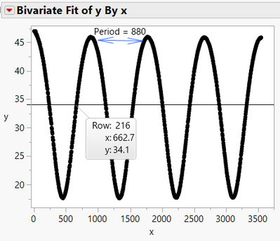
I am struggling with fitting measured data to a trigonometric Ksin(ax+b)+c function. this is the nature of my process and I am looking for an automatic way to fit it by jsl code.
I've wrote a code that normalize the data so the oscillation is between -1 and 1.
At the end I would like to get a and b constants (K and c as well but it is much easier)
attached example for my data type.
BR,
Yoav
Accepted Solutions
- Mark as New
- Bookmark
- Subscribe
- Mute
- Subscribe to RSS Feed
- Get Direct Link
- Report Inappropriate Content
Re: Data Fitting to Trigonometric Functions
Here's how to get an estimate of the a parameter using the FFT function. The comments about seconds and hours are assuming the data was collected about every 4 seconds for about an hour; the FFT doesn't care about the units. The FFT bins the frequencies in the data such that the first bin after the DC offset bin represents the lowest frequency that can make one complete cycle in the input data, the next bin is 2 complete cycles, ... the middle bin is ndata/2 cycles. The bins after than are a mirror of the first.
dt = Open( "z:\example data.jmp" );
// by hand, I made a formula column to look at x-lag(x) and
// decided the first 79 and last 8 were not representative...
rowstart = 80;
rowstop = 937;
timeStart = dt:x[rowstart];
timeStop = dt:x[rowstop];
ydata = dt[rowstart :: rowstop, {y}]; // throw away a few with irregular time
{r, i} = FFT( {ydata} );
nBins = N Items( r );

sampleRate = (timeStop - timeStart) / (nBins - 1); // imagine there were only 2 bins...thus -1.
// the samplerate is ~4 seconds/sample...
// the highest frequency this can resolve is 1 cycle/ 8 seconds. (.125 Hz)
// frequencies higher than that will cause aliasing unless they are filtered out before this.
// the bin [nBins/2] represents the maximum frequency that can be resolved
lastBinFrequency = 1 / (2 * sampleRate); // ~ 0.125 Hz

// the first bin [1] is the DC, or offset from 0, component. We'll ignore it.
// the next bin [2] represents the frequency that has one cycle over the length of the data.
// the lowest non-DC frequency is one cycle per hour (the length of time the data was collected).
binWidth = 1 / (timeStop - timeStart); // ~0.0003Hz, or ~1 cycle per hour
// note: lastBinFrequency == (nbins-1)*binWidth/2 -- each bin is this wide, in frequency

// the remaining bins are a mirror of the first and ignored.

// combine real and imaginary bin components to get an amplitude
p = Sqrt( r ^ 2 + i ^ 2 );
dtGraph2 = As Table( ((rowstart :: rowstop) - rowstart)` || p );
dtGraph2 << Graph Builder(
	Size( 1300, 500 ),
	Show Control Panel( 0 ),
	Show Legend( 0 ),
	Variables( X( :Col1 ), Y( :Col2 ) ),
	Elements( Points( X, Y, Legend( 5 ) ) ),
	SendToReport(
		Dispatch( {}, "Col1", ScaleBox, {Format( "Best", 12 ), Min( 0 ), Max( nBins / 2 ), Inc( 100 ), Minor Ticks( 4 )} ),
		Dispatch( {}, "Col2", ScaleBox, {Format( "Best", 12 ), Min( 0 ), Max( 30000 ), Inc( 5000 ), Minor Ticks( 1 )} ),
		Dispatch( {}, "graph title", TextEditBox, {Set Text( "FFT Bins" )} ),
		Dispatch( {}, "X title", TextEditBox, {Set Text( "bin number" )} ),
		Dispatch( {}, "Y title", TextEditBox, {Set Text( "size" )} )
	)
);
// there is a stong DC component in this data (all values > 0) so bin 1 is the max.
If( Loc Max( p ) != 1,
	Throw( "something odd" )
);
p[1] = 0; // clear the DC value

// next max after DC:
maxBinIndex = Loc Max( p ); // 5. the data repeats about (5-1)==4 times in this frame.
Write(
	"\!nBiggest frequency component at ",
	binWidth * (maxBinIndex - 1),
	" Hz or ",
	Round( 1 / (binWidth * (maxBinIndex - 1)) ),
	" seconds per cycle"
);

// where does a==.007 come from?
secondsPerCycle =  1 / (binWidth * (maxBinIndex - 1));
totalSeconds = timeStop-timeStart;
cyclesInSample = totalSeconds/secondsPerCycle;//about 4
timerange = timeStop-timeStart;
a_from_fft = cyclesInSample*2*pi()/timerange; // .0073...
show(a_from_fft);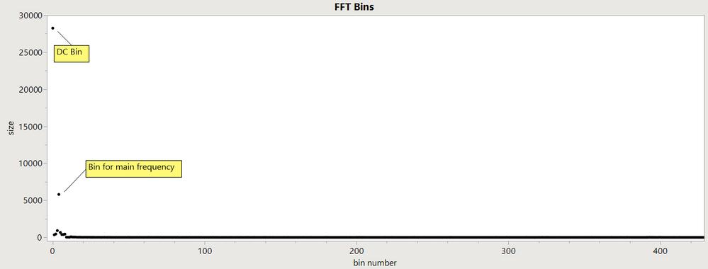
Biggest frequency component at 0.00116448326055313 Hz or 859 seconds per cycle
a_from_fft = 0.007316664113164;
The DC component is related to the mean of the data, the c value.
- Mark as New
- Bookmark
- Subscribe
- Mute
- Subscribe to RSS Feed
- Get Direct Link
- Report Inappropriate Content
Re: Data Fitting to Trigonometric Functions
I think it helps to use what I refer to as the standard form of a sine function: Y = K*sin(A*(x - B)) + C.
In your data:
K = 1/2 of the range of values
A = 2*pi / period
B = shift to the right from 0 to the starting point of the sine wave
C = mean of your Y values
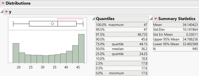
Starting estimates for the nonlinear regression can be found using these definitions from the Distribution platform and Graph Builder:
K = 1/2 * (Max - Min) = 1/2*(47 - 17.6) = 14.7
A = 2 * 3.14 / 880 = 0.007
B = 662
C = 34.1
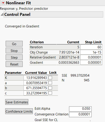
The nonlinear regression converges very quickly using this approach. The model converged in 5 iterations using these values. See below
- Mark as New
- Bookmark
- Subscribe
- Mute
- Subscribe to RSS Feed
- Get Direct Link
- Report Inappropriate Content
Re: Data Fitting to Trigonometric Functions
You could use a zero crossing detector, which would be a small bit of JSL to walk through your data and notice every time the data goes from negative to positive. That's the start of a sine wave cycle. The distance to the next zero crossing is the period.
You might have issues with noisy data that appears to cross several times.
The zero crossing is easier to detect than peaks.
I used that idea in Glitch .
- Mark as New
- Bookmark
- Subscribe
- Mute
- Subscribe to RSS Feed
- Get Direct Link
- Report Inappropriate Content
Re: Data Fitting to Trigonometric Functions
I don't know if this is what you want, but you can solve this using the nonlinear platform. Attached is your data, along with a predictor column (using the parameters to estimate) and a script which solves for those parameters. I will admit that it took me quite a while to get initial guesses for the parameters that allowed the solution to converge (probably due to my lack of familiarity with the sine function - it's been a long long time since I worked with such functions). But, conceptually, the nonlinear platform will accomplish what you want.
- Mark as New
- Bookmark
- Subscribe
- Mute
- Subscribe to RSS Feed
- Get Direct Link
- Report Inappropriate Content
Re: Data Fitting to Trigonometric Functions
Here's how to get an estimate of the a parameter using the FFT function. The comments about seconds and hours are assuming the data was collected about every 4 seconds for about an hour; the FFT doesn't care about the units. The FFT bins the frequencies in the data such that the first bin after the DC offset bin represents the lowest frequency that can make one complete cycle in the input data, the next bin is 2 complete cycles, ... the middle bin is ndata/2 cycles. The bins after than are a mirror of the first.
dt = Open( "z:\example data.jmp" );
// by hand, I made a formula column to look at x-lag(x) and
// decided the first 79 and last 8 were not representative...
rowstart = 80;
rowstop = 937;
timeStart = dt:x[rowstart];
timeStop = dt:x[rowstop];
ydata = dt[rowstart :: rowstop, {y}]; // throw away a few with irregular time
{r, i} = FFT( {ydata} );
nBins = N Items( r );

sampleRate = (timeStop - timeStart) / (nBins - 1); // imagine there were only 2 bins...thus -1.
// the samplerate is ~4 seconds/sample...
// the highest frequency this can resolve is 1 cycle/ 8 seconds. (.125 Hz)
// frequencies higher than that will cause aliasing unless they are filtered out before this.
// the bin [nBins/2] represents the maximum frequency that can be resolved
lastBinFrequency = 1 / (2 * sampleRate); // ~ 0.125 Hz

// the first bin [1] is the DC, or offset from 0, component. We'll ignore it.
// the next bin [2] represents the frequency that has one cycle over the length of the data.
// the lowest non-DC frequency is one cycle per hour (the length of time the data was collected).
binWidth = 1 / (timeStop - timeStart); // ~0.0003Hz, or ~1 cycle per hour
// note: lastBinFrequency == (nbins-1)*binWidth/2 -- each bin is this wide, in frequency

// the remaining bins are a mirror of the first and ignored.

// combine real and imaginary bin components to get an amplitude
p = Sqrt( r ^ 2 + i ^ 2 );
dtGraph2 = As Table( ((rowstart :: rowstop) - rowstart)` || p );
dtGraph2 << Graph Builder(
	Size( 1300, 500 ),
	Show Control Panel( 0 ),
	Show Legend( 0 ),
	Variables( X( :Col1 ), Y( :Col2 ) ),
	Elements( Points( X, Y, Legend( 5 ) ) ),
	SendToReport(
		Dispatch( {}, "Col1", ScaleBox, {Format( "Best", 12 ), Min( 0 ), Max( nBins / 2 ), Inc( 100 ), Minor Ticks( 4 )} ),
		Dispatch( {}, "Col2", ScaleBox, {Format( "Best", 12 ), Min( 0 ), Max( 30000 ), Inc( 5000 ), Minor Ticks( 1 )} ),
		Dispatch( {}, "graph title", TextEditBox, {Set Text( "FFT Bins" )} ),
		Dispatch( {}, "X title", TextEditBox, {Set Text( "bin number" )} ),
		Dispatch( {}, "Y title", TextEditBox, {Set Text( "size" )} )
	)
);
// there is a stong DC component in this data (all values > 0) so bin 1 is the max.
If( Loc Max( p ) != 1,
	Throw( "something odd" )
);
p[1] = 0; // clear the DC value

// next max after DC:
maxBinIndex = Loc Max( p ); // 5. the data repeats about (5-1)==4 times in this frame.
Write(
	"\!nBiggest frequency component at ",
	binWidth * (maxBinIndex - 1),
	" Hz or ",
	Round( 1 / (binWidth * (maxBinIndex - 1)) ),
	" seconds per cycle"
);

// where does a==.007 come from?
secondsPerCycle =  1 / (binWidth * (maxBinIndex - 1));
totalSeconds = timeStop-timeStart;
cyclesInSample = totalSeconds/secondsPerCycle;//about 4
timerange = timeStop-timeStart;
a_from_fft = cyclesInSample*2*pi()/timerange; // .0073...
show(a_from_fft);
Biggest frequency component at 0.00116448326055313 Hz or 859 seconds per cycle
a_from_fft = 0.007316664113164;
The DC component is related to the mean of the data, the c value.
- Mark as New
- Bookmark
- Subscribe
- Mute
- Subscribe to RSS Feed
- Get Direct Link
- Report Inappropriate Content
Re: Data Fitting to Trigonometric Functions
I think it helps to use what I refer to as the standard form of a sine function: Y = K*sin(A*(x - B)) + C.
In your data:
K = 1/2 of the range of values
A = 2*pi / period
B = shift to the right from 0 to the starting point of the sine wave
C = mean of your Y values
Starting estimates for the nonlinear regression can be found using these definitions from the Distribution platform and Graph Builder:
K = 1/2 * (Max - Min) = 1/2*(47 - 17.6) = 14.7
A = 2 * 3.14 / 880 = 0.007
B = 662
C = 34.1
The nonlinear regression converges very quickly using this approach. The model converged in 5 iterations using these values. See below
- Mark as New
- Bookmark
- Subscribe
- Mute
- Subscribe to RSS Feed
- Get Direct Link
- Report Inappropriate Content
Re: Data Fitting to Trigonometric Functions
Great, that is exactly the intuition I was lacking. Instead, I manipulated the parameter values in the nonlinear platform until the graph looked close to the data, but knowing what the parameters represent (and getting good initial guesses from the data) is a much superior way to go.
- Mark as New
- Bookmark
- Subscribe
- Mute
- Subscribe to RSS Feed
- Get Direct Link
- Report Inappropriate Content
Re: Data Fitting to Trigonometric Functions
Hi, Thanks all for the time you spend on it. This is looks like great approach for my application. but- how did you got "automatically" the period length? I didn't got that..
Yoav
- Mark as New
- Bookmark
- Subscribe
- Mute
- Subscribe to RSS Feed
- Get Direct Link
- Report Inappropriate Content
Re: Data Fitting to Trigonometric Functions
You could use a zero crossing detector, which would be a small bit of JSL to walk through your data and notice every time the data goes from negative to positive. That's the start of a sine wave cycle. The distance to the next zero crossing is the period.
You might have issues with noisy data that appears to cross several times.
The zero crossing is easier to detect than peaks.
I used that idea in Glitch .
Recommended Articles
- © 2026 JMP Statistical Discovery LLC. All Rights Reserved.
- Terms of Use
- Privacy Statement
- Contact Us


