Distribution new features for JMP 17

[#1]

JMP 17 brings new features to the Distribution platform. 

• Detection limits column property support. 
• Confidence intervals in QQ and PP plots.
• New platform preferences command. 

Keep reading to learn more about these new features.

Example

Let’s use an example to demonstrate the new features. Open Metacrate Limit of Detection DOE.jmp found in the Design Experiment sample data folder.

dt=Open("$SAMPLE_DATA/Design Experiment/Metacrate Limit of Detection DOE.jmp");

Take a look at the Metacrate column. This column contains measurements of a pesticide (metacrate) found in water samples. 

Detection Limits

Small amounts are hard to measure. Measuring devices have only a certain amount of accuracy. Detection limits define bounds beyond which the response cannot be measured. If you are unfamiliar with detection limits, view the following JMP Discovery Summit poster by Clay Barker, the co-developer of the platform, to learn more. This presentation not only discusses detection limits but also shows what happens when you ignore them when analyzing your data.

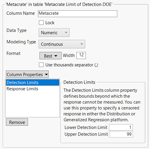
The data table shows that Metacrate has a Detection Limits column property with a Lower Detection Limit of 1 and an Upper Detection Limit of 99.  

This means the measurement device cannot measure metacrate values below 1 or above 99. The values for Metacrate that are colored red in the data table indicate censored values because they are below 1, which is the smallest value that the measurement device can measure. 

The first step to analyzing censored data using the distribution platform is to fit a distribution.  Run the following:

Distribution( Continuous Distribution( Column( :Metacrate ) ) );

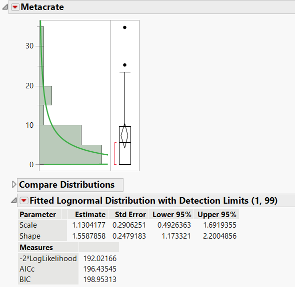
Under the Continuous Fit option from the red triangle menu, you will notice only six options. The first five options are fits that deal with censored data and the detection limit column property. For this example, let’s choose the Lognormal fit since it often works well with impurity-type data.

You will notice the new outline node, Fitted Lognormal Distribution with Detection Limits (1, 99). This indicates that the detection limits were used when fitting the lognormal distribution. 

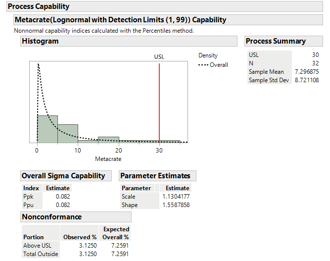
Capability analysis selected from a fitted distribution will also use the detection limits column property. Click the red triangle next to Fitted Lognormal Distribution with Detection Limits (1, 99) and choose Process Capability. Enter an upper specification limit of 30.  Click OK.

You will be presented with an outline node, Metacrate(Lognormal with Detection Limits (1, 99)) Capability, indicating that the capability analysis used the detection limits column property. You can compare these results to results from ignoring the detection limits column property and see how much of a difference it makes.

Confidence Intervals in QQ and PP Plots

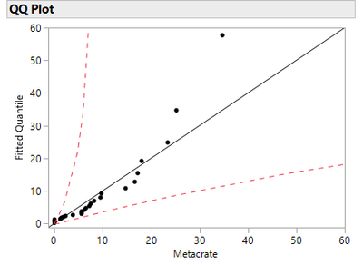
Confidence intervals are now in QQ and PP Plots. Click the red triangle next to Fitted Lognormal Distribution with Detection Limits (1, 99) and select QQ Plot.

You can see dashed lines for the 95 percent confidence interval, which are helpful in determining the accuracy of your fit.

Platform Preferences

The Platform Preferences option in the red triangle menu is new for all platforms. This option contains a submenu with Go to and Save Changes to. For this example, the Go to option takes you to the platform preferences for Distribution. The Save Changes to option will open a dialog that allows you to alter any non-default platform preferences for Distribution.

Conclusion

New features are in Distribution. 

• Detection limits column property support. 
• Confidence intervals in QQ and PP plots.
• New platform preferences command.

These new additions make the distribution platform more complete.