- New to JMP? Let the Data Analysis Director guide you through selecting an analysis task, an analysis goal, and a data type. Available now in the JMP Marketplace!
- See how to install JMP Marketplace extensions to customize and enhance JMP.
JMP Blog
A blog for anyone curious about data visualization, design of experiments, statistics, predictive modeling, and more- JMP User Community
- :
- Blogs
- :
- JMP Blog
- :
- Text analysis in the social sciences: A new spectrum of possibilities
- Subscribe to RSS Feed
- Mark as New
- Mark as Read
- Bookmark
- Subscribe
- Printer Friendly Page
- Report Inappropriate Content
Computer scientists have long profited from methodology that allows them to extract information from a variety of text documents. Their methodology not only tallies up terms and phrases in texts, but it also uncovers structure and provides insight into the content of texts. On the other hand, most social scientists — who have plenty of text data in comment fields of surveys, interview transcripts, etc. — don’t seem to rely on these methods (those who study language or collaborate with computer scientists are the rare exceptions).
In this post, I encourage social scientists to explore the spectrum of possibilities that text analysis can afford. I do so by providing a brief explanation of two text analytic techniques: Latent Semantic Analysis (LSA) and Topic Analysis (TA). As it will soon be obvious, social scientists with a background on multivariate statistics will be able to use, apply, and interpret LSA and TA effortlessly (it might just take this post to get you up and running!) My explanation relies on two statistical techniques that are well-known in the social sciences: Principal Component Analysis (PCA) and Factor Analysis (FA).
A Review of Principal Components Analysis
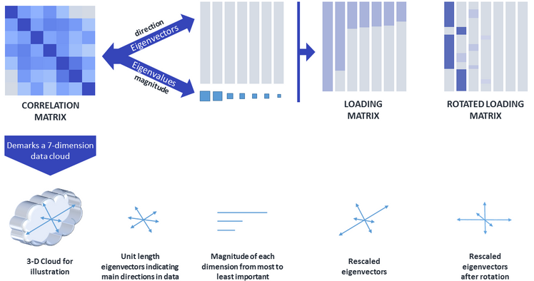
PCA is a method that allows us to identify and extract uncorrelated dimensions of maximal variability from our data. This is done through an eigenvalue decomposition of the correlation matrix of the data. Figure 1 depicts the steps involved in the eigenvalue decomposition and ensuing steps to aid in interpretation of the PCA (note the figure is oversimplified to facilitate this review).

The correlation matrix represents a “data cloud” in a multidimensional space. The eigenvalue decomposition helps identify the main dimensions that are perpendicular to each other within this cloud and produces two key pieces of information: the eigenvectors, which are indicative of the directions of the main dimensions, and the eigenvalues, which identify the magnitude of each dimension and are the variances of the dimensions. If only a couple dimensions capture most of the variability in the data (i.e., the first two eigenvalues are large with respect to all others), then analysts might choose to retain the first two eigenvectors and eigenvalues to reduce the number of variables they have to analyze. All eigenvectors are of unit length but can be “resized” using the information provided by the eigenvalues. These rescaled eigenvectors are known as loadings.
Loading vectors have variability equal to their corresponding eigenvalue. Moreover, loading coefficients are correlation coefficients that describe the association between the dimension (principal component) and the corresponding variable. For this reason, loadings are critical for understanding what a principal component represents. However, a loading matrix can have a difficult pattern to discern, such as loadings of moderate magnitude across several dimensions (see Loading Matrix in Figure 1). Thus, analysts might choose to rotate the loading matrix in an effort to improve interpretation of the components. Most often, an orthogonal rotation is employed (e.g., Varimax), which tends to result in a simple pattern of loadings (termed “simple structure” by Thurstone, 1947). That is, the loadings are very high for a given component and nearly zero for all other components. Simple structure of the rotated loading matrix (see Figure 1) helps identify with clarity what each principal component represents.
Principal Component Analysis == Latent Semantic Analysis
Now that PCA is fresh in your mind, the good news is that latent semantic analysis (LSA) is simply PCA done on a correlation matrix of text terms (but without any rotations involved). In other words, the variables in the analysis are columns that indicate the incidence of a term across text documents. This set of variables is called a document term matrix (DTM; see Figure 2), which has as many columns as there are terms in the documents and as many rows as there are documents. If we want a binary DTM, each cell entry can be a 0 or 1 depending on whether the given term is in the given document. A frequency DTM requires each entry to be a count of the number of times the term appears in the given document. There are other ways to construct the DTM; a preferred method in the literature (Ramos, 2003) is called TF-IDF (term frequency-inverse document frequency), which you can implement in JMP with the click of a button!

Notice the first document in Figure 2 has the word “from” and yet that term doesn’t show up in the DTM. This is because there are important preliminary steps to creating a DTM. Let’s see those next!
Setting up Text Data for Analysis
Text analysis starts by identifying the unit of measurement. Specifically, you have to determine what will constitute a “document.” A document can be a sentence, paragraph, article, or book, among many other choices. The next step involves identifying relevant terms across the documents. You do this by filtering out “stop words” (those extremely common words that aren’t likely to help unveil the structure in the text corpus, such as “the,” “and,” “from,” “is,” “of,” etc.). Moreover, you might choose to condense similar terms into one. For example, the columns “analysis” and “analytics” in Figure 2 are redundant and can be combined into one column “analy.” This is called stemming. Finally, not all words in a text should be split apart. “Social scientists” in the first row of Figure 2 is one example. You can combine these words into one term prior to creating the DTM (you can do the same with phrases like “once upon a time”).
All steps above are critical for a solid analysis. Luckily, the Text Explorer platform in JMP makes these tasks a breeze! Under the Analyze > Text Explorer menu, assign the column in the data table containing the documents as the Text Column (see Figure 3). You can also customize options for stemming in the launch window. After launching Text Explorer, you can further select phrases to be considered as terms.

With all preliminary steps completed, you can create the DTM and carry out a PCA with it. However, depending on how large your DTM is (and they tend to be quite large), a PCA as I described above can take a long time to run and require lots of memory. Fortunately, JMP uses singular value decomposition in place of eigenvalue decomposition to make this analysis very efficient! In a future post, I’ll explain the equivalencies between eigenvalue decomposition and singular value decomposition, but for now, you’ll have to trust me that both approaches will lead to the same results.
Topic Analysis
Another valuable text analysis technique is Topic Analysis (TA). This technique can also be easily translated to social scientists by clarifying that TA is simply PCA with a Varimax rotation of the loading matrix. Similar to LSA, TA is carried out with singular value decomposition instead of eigenvalue decomposition to make it more efficient. Results from TA are likely to be easier to interpret than those from LSA because of the rotation of the loadings. The topics will be the main dimensions of variability in your text data. The loadings allow you to interpret what the topic represents. Moreover, topic (or component) scores can be computed and used in secondary analyses.
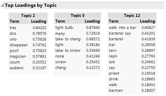
To give a sense of what TA can do, I performed TA on a data set of 231,657 jokes*. To avoid offending any readers, I’m only showing the results of three topics that came up from the analysis (Figure 4).

Readers might agree that there’s a clear distinction between the types of jokes each of the topics in Figure 4 represent. For more compelling examples of text analysis, see this post on predicting future stock prices, or read a recent publication using social media data (Kern et al., 2016). Or watch this video.
Remarks on Factor Analysis
In the opening section, I said I’d rely on social scientists’ knowledge of PCA and FA. But so far I’ve only discussed PCA. If your training was at all similar to mine, you know there are important differences between PCA and FA. In a previous post, I described those differences, but I also mentioned one key similarity: Results from PCA and FA become increasingly similar as the data matrix under consideration grows in size (if you want a refresher on FA, I recommend you read the post). Indeed, in text analysis, data matrices tend to be very large. In the Sample Document Term Matrix above, the DTM has 10 variables already! And the joke example has a DTM with 4,316 variables!). Thus, topics or components from LSA and TA can be thought of as latent variable approximations and can be used effectively to tackle a myriad of research questions!
To Close…
Too often, we allow our statistical tool kit to determine the design and analysis of our research (sometimes inadvertently!). Thus, I hope this post opens the door to new research questions in the social sciences (and other fields) that can be uniquely tackled with text analytics.
Key Points
- Text analysis is underutilized in the social sciences despite the fact that it relies on statistical techniques that are well-known to social scientists.
- Latent semantic analysis is equivalent to principal components analysis done on a document term matrix.
- A document term matrix has as many rows as there are documents and as many columns as there are terms in the documents. Cells contain the incidence of terms in a given document.
- Topic analysis is equivalent to principal components analysis with a rotation of the component loadings to aid interpretation of the topics. But note that some clustering methods are sometimes also described as topic analysis.
- Because document term matrices tend to be quite large, social scientists can think of principal components as pretty good approximations of latent variables or latent topics.
There’s much more to say about text analysis! I suggest starting with this on-demand webcast, which does a great job at describing many more details. You can also see my post about the Text Explorer platform in JMP, especially the Rosetta Stone section, which clarifies more linkages between PCA and LSA/TA.
References
- Kern, M. L., Park, G., Eichstaedt, J. C., Schwartz, H. A., Sap, M., Smith, L. K., & Ungar, L. H. (2016). Gaining insights from social media language: Methodologies and challenges. Psychological Methods. Advance online publication. http://dx.doi.org/10.1037/met0000091
- Ramos, J. (2003, December). Using tf-idf to determine word relevance in document queries. In Proceedings of the first instructional conference on machine learning (Vol. 242, pp. 133-142).
- Thurstone, L. L. (1947). Multiple factor analysis. Chicago: University of Chicago Press, 1947.
* Thanks to amoudgl who made this file freely available here: https://github.com/amoudgl/short-jokes-dataset
- © 2026 JMP Statistical Discovery LLC. All Rights Reserved.
- Terms of Use
- Privacy Statement
- Contact Us

You must be a registered user to add a comment. If you've already registered, sign in. Otherwise, register and sign in.