- New to JMP? Let the Data Analysis Director guide you through selecting an analysis task, an analysis goal, and a data type. Available now in the JMP Marketplace!
- See how to install JMP Marketplace extensions to customize and enhance JMP.
JMP Blog
A blog for anyone curious about data visualization, design of experiments, statistics, predictive modeling, and more- JMP User Community
- :
- Blogs
- :
- JMP Blog
- :
- Principal components or factor analysis?
- Subscribe to RSS Feed
- Mark as New
- Mark as Read
- Bookmark
- Subscribe
- Printer Friendly Page
- Report Inappropriate Content
Should I use principal components analysis (PCA) or Exploratory Factor Analysis (EFA) for my work? This is a common question that analysts working with multivariate data, such as social scientists, consumer researchers, or engineers, face on a regular basis.
In this post, I share my favorite example for explaining a key difference between PCA and EFA. This distinction opens the door to explaining other important differences and is helpful when figuring out which technique is most appropriate for a given application. Choosing improperly might mean misleading results or incorrect understanding of the data.
An Illustrative Example
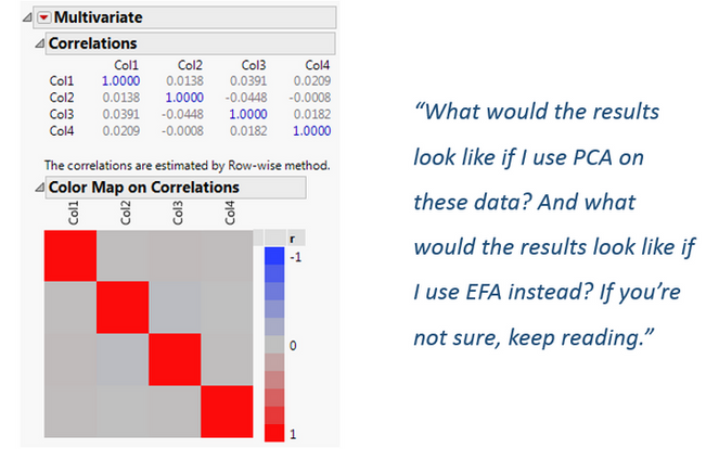
Let’s start by creating some data that follow a standard normal distribution (a JSL script for all analyses in this post is attached if you want to follow along). Specifically, I create a data table with 1,000 observations on four variables that are uncorrelated with each other.
We can use the Multivariate platform in JMP to look at the correlations between variables and confirm they are independent. I particularly like to use the Color Map on Correlations to illustrate the null correlations in the off-diagonal:

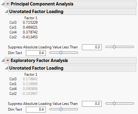
Let’s use the Factor Analysis platform in JMP to perform simultaneously a PCA and an EFA on these data. I’ll retain one component/factor only because we have a small number of variables. This also eliminates the need for any rotation.
The component or factor loadings from the analyses are critical to help us understand what the component or factor represents; variables with high loadings (usually defined as .4 in absolute value or higher because this suggests at least 16% of the measured variable variance overlaps with the variance of the factor) are most representative of the component or factor. Below, we can compare the resulting component loadings (displayed first) against the factor loadings (displayed second).

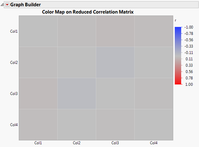
We can see the results are strikingly different! PCA gave us three loadings greater than .4 in absolute value whereas EFA didn’t give any. Why? Because when we do EFA we are implicitly requesting an analysis on a reduced correlation matrix, for which the ones in the diagonal have been replaced by squared multiple correlations (SMC). Indeed, a quick look at the Color Map on Correlations of the reduced correlation matrix sheds light on why one would obtain such different results:

Every entry in the reduced correlation matrix, in this example, is very small (nearly zero! The actual values are 0.002, 0.002, 0.004, and 0.001). An eigenvalue decomposition of the full correlation matrix (Figure 1) is done in PCA, yet for EFA, the eigenvalue decomposition is done on the reduced correlation matrix (Figure 3). Differences in the data analyzed help explain differences across analyses, but none of this tells us what the differences mean from a practical point of view….
Practical Meaning of Analyzing a Full vs. Reduced Correlation Matrix
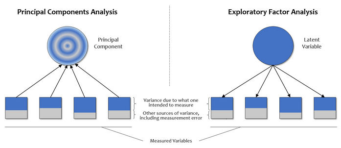
PCA and EFA have different goals: PCA is a technique for reducing the dimensionality of one’s data, whereas EFA is a technique for identifying and measuring variables that cannot be measured directly (i.e., latent variables or factors). Thus, in PCA all of the variance in the data — reflected by the full correlation matrix — is used to attain a solution, and the resulting components are a mix of what the variables intended to measure and other sources of variance such as measurement error (see left panel of Figure 4).
By contrast, in EFA not all of the variance in the data comes from the underlying latent variable (see right panel of Figure 4). This feature is reflected in the EFA algorithm by “reducing” the correlation matrix with the SMC values. This is appropriate because a SMC is the estimate of the variance that the underlying factor(s) explain in a given variable (aka communality). If we carried out EFA with unities in the diagonal, then we would be implicitly saying the factors explain all the variance in the measured variables, and we would be doing PCA rather than EFA.

Figure 4 also illustrates another important distinction between PCA and EFA. Note the arrows in PCA are pointing from the measured variables to the principal component, and in EFA it’s the other way around. The arrows represent causal relations, such that the variability in measured variables in PCA cause the variance in the principal component. This is in contrast to EFA, where the latent factor is seen as causing the variability and pattern of correlations among measured variables (Marcoulides & Hershberger, 1997).
In the interest of clarity, it’s important I outline a few more observations. First, most multivariate data are correlated to some degree, so differences between PCA and EFA don’t tend to be as marked as the ones in this example. Second, as the number of variables involved in the analysis grows, results from PCA and EFA become more and more similar. Researchers have argued that analyses with at least 40 variables lead to minor differences (Snook & Gorsuch, 1989). Third, if the communality of measured variables is high (i.e., approaches 1), then the results between PCA and EFA are also similar. Finally, this favorite example of mine relies on using the “Principal Axis” factoring method, but other estimation methods exist for which results would vary. All of these observations must be taken into account when analysts make the choice between EFA and PCA. But perhaps most importantly for psychometricians (those who developed EFA in the first place) is the fact that EFA posits a theory about the variables being analyzed; a theory that dates back to Spearman (1904) and suggests unobserved factors determine what we’re able to measure directly.
I list some key points below, but note that an excellent source for continuing to learn about this topic is Widaman (2007).
Key Points
- PCA is useful for reducing the number of variables while retaining the most amount of information in the data, whereas EFA is useful for measuring unobserved (latent), error-free variables.
- When variables don’t have anything in common, as in the example above, EFA won’t find a well-defined underlying factor, but PCA will find a well-defined principal component that explains the maximal amount of variance in the data.
- When the goal is to measure an error-free latent variable but PCA is used, the component loadings will most likely be higher than they would’ve been if EFA was used. This would mislead analysts into thinking they have a well-defined, error-free factor when in fact they have a well-defined component that’s an amalgam of all the sources of variance in the data.
- When the goal is to get a small subset of variables that retain the most amount of variability in the data but EFA is used, the factor loadings will likely be lower than they would’ve been if PCA was used. This would mislead analysts into thinking they kept the maximal amount of variance in the data when in fact they kept the variance that’s in common across the measured variables.
- The difference between PCA and EFA is relevant to analyses that extend these techniques, such as structural equation modeling (SEM). Partial Least Squares SEM (PLS-SEM) models structural relations between component variables, whereas covariance-based SEM models structural relations between error-free latent variables.
References
Marcoulides, G. A., & Hershberger, S. L. (1997). Multivariate statistical methods: A first course. Psychology Press.
Snook, S. C., & Gorsuch, R. L. (1989). Component analysis versus common factor analysis: A Monte Carlo study. Psychological Bulletin, 106, 148-154.
Spearman, C. (1904). "General intelligence," objectively determined and measured. The American Journal of Psychology, 15, 201-293.
Widaman, K. F. (2007). Common factors versus components: Principals and principles, errors and misconceptions. Factor analysis at 100: Historical developments and future directions, 177-203.
You must be a registered user to add a comment. If you've already registered, sign in. Otherwise, register and sign in.
- © 2026 JMP Statistical Discovery LLC. All Rights Reserved.
- Terms of Use
- Privacy Statement
- Contact Us
