comparison of slopes

[#1]

After running an ANCOVA model with more than two values of the categorical variable, how can I perform pairwise comparisons of slopes?

Hillary.

[#2]

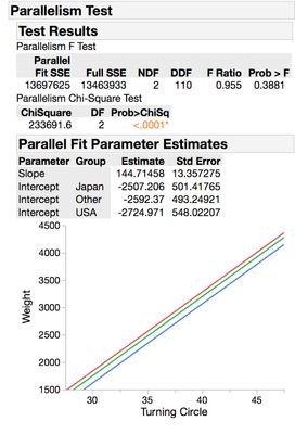
After some digging...the ANOM in the nonlinear platform appears to be comparing the estimates to the "parallel" model where the model for each group has the same shape but is shifted along the x-axis.  So in the case of the example we have been looking at the center line for the slope ANOM of 144.71 is the slope of the model with the same slope but different intercepts for each group.

[#3]

You're correct. I've misunderstood the question and showed the pairwise comparison of the estimated effects of the categorical variable.

[#4]

Julian,

I find this post very useful. However, I am struggling with a question. If the categorical variable has many levels for example 18 in my case, JMP is doing a pairwise comparison of the slopes. Is there anyway to get a multiple comparison through Tukey or other tests to avoid the big error rate by having pair wise comparisons of slope. Thank you

[#5]

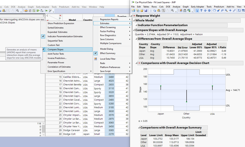
In recent JMP versions, the Fit Model Platform also has a "Compare Slopes" report option under Estimates under the top red triangle in the Fit Model output. 

This report can be used to statistically compare each of the individual slopes (corresponding to each Level of the categorical factor) to the overall average slope, using the Analysis of Means (ANOM) construct in JMP.

Notice how in this example, since none of the three slopes exceed the decision limits of the test (UDL, LDL), we can assert that none of the slopes are statistically significantly different than the overall average slope; therefore, we can infer that none of the slopes are different from each other.  This conclusion squares up nicely with what we can assert when conducting pairwise comparisons to compare the slopes as detailed above.

For example, when comparing Japan to USA, we can assert that we do not have evidence to reject the null hypothesis that the slopes are the same, given the Pairwise comparisons test p-value obtained = 0.9985.  We can make similar statements when comparing Other vs USA, and Japan vs Other (where p= 0.2193 and p=0.2204, respectively).

Also notice that the "Group Mean" as detailed in the 'Comparisons with Overall Average Summary' header at the bottom of the report is just the slope corresponding to the particular level of Country.  For example, the slope corresponding to Japan is 155.5177 and that corresponding to Other is 113.0713.  Japan - Other = 155.5177 - 113.0713 = 42.4464 which rounds to 42.45, identical to the analysis above. 

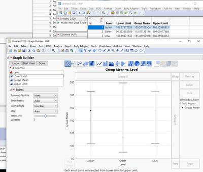
Finally, notice that the confidence limits on the observed slopes are indicated by "Lower Limit" and "Upper Limit" respectively.  We can graph the observed slopes and their confidence limits in JMP using Graph Builder after right clicking to make into a data table. 

By dragging Upper Limit and Lower Limit into the Limits role in Graph Builder, Group Mean into the Y role and Level into X role, we obtain the following graph which is just a graphical representation of the table:

Since all three confidence intervals overlap with each other, we can assert based on the relation between confidence intervals and tests of significance (see Ch. 21 of Experimental Statistics by Mary Gibbons Natrella from the National Bureau of Standards), that we do not have evidence that the Slopes are different from each other (at the 0.05 alpha level, since these limits are constructed with 95% confidence).