- New to JMP? Let the Data Analysis Director guide you through selecting an analysis task, an analysis goal, and a data type. Available now in the JMP Marketplace!
- See how to install JMP Marketplace extensions to customize and enhance JMP.
- Subscribe to RSS Feed
- Mark Topic as New
- Mark Topic as Read
- Float this Topic for Current User
- Bookmark
- Subscribe
- Mute
- Printer Friendly Page
Discussions
Solve problems, and share tips and tricks with other JMP users.- JMP User Community
- :
- Discussions
- :
- Re: comparison of slopes
- Mark as New
- Bookmark
- Subscribe
- Mute
- Subscribe to RSS Feed
- Get Direct Link
- Report Inappropriate Content
comparison of slopes
After running an ANCOVA model with more than two values of the categorical variable, how can I perform pairwise comparisons of slopes?
Hillary.
Accepted Solutions
- Mark as New
- Bookmark
- Subscribe
- Mute
- Subscribe to RSS Feed
- Get Direct Link
- Report Inappropriate Content
Re: comparison of slopes
Hi hillaryvoet,
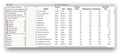
If I'm understanding your question correctly, you have a regression with a categorical variable (X1) and continuous variable (X2) and the interaction between them predicting a continuous variable (Y). Your categorical variable (X1) has more than two levels, and you have a statistically significant interaction between X1 and X2 and would like to follow-up on that to see for which groups the regression of Y on to X2 differs. The methods listed by others here don't seem to be testing the pairwise differences in slopes, but rather the pairwise difference in means, assuming a mean level on the continuous regressor (X2). There is a way to get the tests you want, but it'll take a few extra steps. I'll use the Car Physical Data sample dataset for this example.
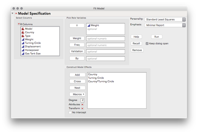
First I will fit a model like you're working with. I predict Weight on the basis of Country and Turning circle, and their interaction.
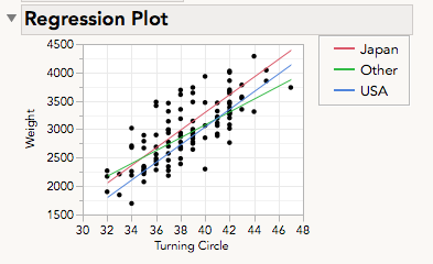
In the regression plot we can see directly what you're asking for, three tests of the differences in slopes between each pair, Japan/Other, Japan/USA, Other/USA.
Tests produced under Effect Details for the factor of Country, (for instance LSMeans Differences Student's t), are not tests of slope differences, but are tests of whether the mean weight of cars differ for those countries assuming the mean level of turning circle.
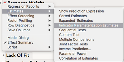
To reveal a test of slopes, we will go to the top-most Red Triangle > Estimates > Indicator Parameterization Estimates
This will show a table of parameter estimates based on an indicator parameterization (as opposed to effects coding, which is what the regular parameter estimates table is based on) which means the LAST level of your categorical factor is used as a reference category, and estimates are differences from that reference category. This will be useful for us.
Notice that we see no estimates with USA. That's because USA is our reference category, so all estimates are differences from what was estimated for the USA. Country[Japan], with the estimate of 256.78, is how much Japan differs from the USA in terms of weight on average. Notice that is the same thing we saw above in the ordered differences report table.
If we look at the interaction parameter estimates we can use the same logic: Country[Japan]*(Turning Circle-38.5862), and the associated estimates, is how the slope for Japan differs from the slope for the USA (by the way, the slope for the USA is listed under "Turning Circle" since it's the reference category, so 155.46 is the USA). Notice that the slope for Japan is nearly the same as the slope for the USA -- different by only a value of 0.06, p = 0.9985. The slope for Other differs from the USA by -42.38, p = 0.2193.
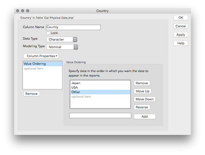
So we're almost there. We're missing one test, Japan vs Other. To get this we need to make JMP treat Japan, or Other, as the reference category, and then rerun this analysis. I'm going to choose to treat Other as the reference category. To change the reference category we'll change the Value Ordering property for the column Country. Right click on the column in the table and go to Column Info. Click on Column Properties, and then select Value Ordering. To change the ordering, select "Other" and click Move Down. The last category listed will be the reference category. Click okay when you're done.
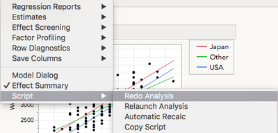
To rerun the model, go to the top-most red triangle of your existing Fit Model output > Script > Redo analysis.
The "Indicator Function Parameterization" now lists the same analyses we saw before, but with "Other" as the reference category.
And now we have our last test, the slope difference between Japan vs Other, which we find in the row "Country[Japan]*(Turning Circle-38.5862)". A difference of 42.45, p = 0.2204.
So we have our three pairwise slope tests.
Japan vs USA, difference = 0.06, p = 0.9985.
Other vs USA, difference = 42.38, p = 0.2193.
Japan vs Other, difference = 42.45, p = 0.2204.
I hope this helps!
- Mark as New
- Bookmark
- Subscribe
- Mute
- Subscribe to RSS Feed
- Get Direct Link
- Report Inappropriate Content
Re: comparison of slopes
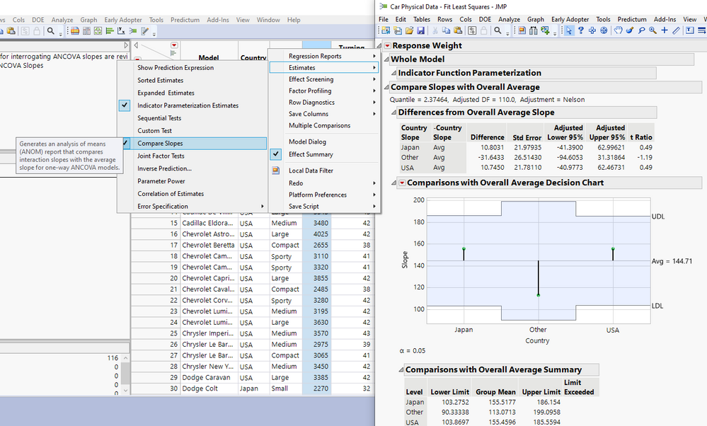
In recent JMP versions, the Fit Model Platform also has a "Compare Slopes" report option under Estimates under the top red triangle in the Fit Model output.
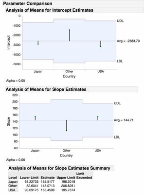
This report can be used to statistically compare each of the individual slopes (corresponding to each Level of the categorical factor) to the overall average slope, using the Analysis of Means (ANOM) construct in JMP.
Notice how in this example, since none of the three slopes exceed the decision limits of the test (UDL, LDL), we can assert that none of the slopes are statistically significantly different than the overall average slope; therefore, we can infer that none of the slopes are different from each other. This conclusion squares up nicely with what we can assert when conducting pairwise comparisons to compare the slopes as detailed above.
For example, when comparing Japan to USA, we can assert that we do not have evidence to reject the null hypothesis that the slopes are the same, given the Pairwise comparisons test p-value obtained = 0.9985. We can make similar statements when comparing Other vs USA, and Japan vs Other (where p= 0.2193 and p=0.2204, respectively).
Also notice that the "Group Mean" as detailed in the 'Comparisons with Overall Average Summary' header at the bottom of the report is just the slope corresponding to the particular level of Country. For example, the slope corresponding to Japan is 155.5177 and that corresponding to Other is 113.0713. Japan - Other = 155.5177 - 113.0713 = 42.4464 which rounds to 42.45, identical to the analysis above.
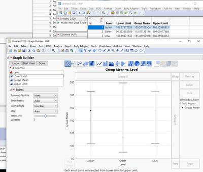
Finally, notice that the confidence limits on the observed slopes are indicated by "Lower Limit" and "Upper Limit" respectively. We can graph the observed slopes and their confidence limits in JMP using Graph Builder after right clicking to make into a data table.
By dragging Upper Limit and Lower Limit into the Limits role in Graph Builder, Group Mean into the Y role and Level into X role, we obtain the following graph which is just a graphical representation of the table:
Since all three confidence intervals overlap with each other, we can assert based on the relation between confidence intervals and tests of significance (see Ch. 21 of Experimental Statistics by Mary Gibbons Natrella from the National Bureau of Standards), that we do not have evidence that the Slopes are different from each other (at the 0.05 alpha level, since these limits are constructed with 95% confidence).
- Mark as New
- Bookmark
- Subscribe
- Mute
- Subscribe to RSS Feed
- Get Direct Link
- Report Inappropriate Content
Re: comparison of slopes
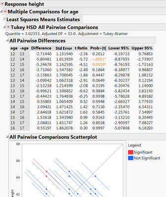
If you use Fit Model's Standard Least Squares for ANCOVA, select Estimates => Multiple Comparisons option from the top red triangle for pairwise comparisons. For more info check out the documentation by scrolling down to All Pairwise Comparisons The following screenshot shows Tukey's all pairwise comparisons for age groups
- Mark as New
- Bookmark
- Subscribe
- Mute
- Subscribe to RSS Feed
- Get Direct Link
- Report Inappropriate Content
Re: comparison of slopes
The ANCOVA is performed by running a model with a categorical variable, a
continuous variable, and – in the case I'm interested in – an interaction
term which tests for equality of slopes. Using Estimates – Multiple
Comparisons gives the differences and significance between the Least Square
Means, notbetween the slopes.
From: jiancao
Sent: Tuesday, May 24, 2016 9:15 PM
To: Hillary Voet <hillary.voet@mail.huji.ac.il>
Subject: Re: - comparison of slopes
JMP User Community
<https://community.jmp.com/?utm_source=JIVE&utm_medium=email&utm_campaign=System%20Email%20Tracking>
comparison of slopes
reply from jiancao
<https://community.jmp.com/people/jiancao?et=watches.email.thread> in
Discussions - View the full discussion
<https://community.jmp.com/message/228740?et=watches.email.thread#228740>
- Mark as New
- Bookmark
- Subscribe
- Mute
- Subscribe to RSS Feed
- Get Direct Link
- Report Inappropriate Content
Re: comparison of slopes
The multiple comparisons test is giving you a comparison of the Least Square Means, but that is the same as the slopes. Consider a case with 2 levels of your categorical variable (let's call it Q) and your continuous variable is called X. Your model is Y = B0 + B1*Q + B2*X + B12*Q*X.
Suppose I fix Q at the first level, 1. My model simplifies to Y = B0 + B1*(1) + B2*X + B12*(1)*X ==> Y = (B0+B1) + (B2+B12)*X.
Notice that the B12 interaction parameter is the adjustment of the slope for the different levels of the categorical variable. Therefore, testing to see if the least squares means of the interaction terms are different is equivalent to testing if the slopes are different. If B12 for level 1 of the categorical variable is different than B12 for level 2 of the categorical variable, then the slopes for those two categories are different.
- Mark as New
- Bookmark
- Subscribe
- Mute
- Subscribe to RSS Feed
- Get Direct Link
- Report Inappropriate Content
Re: comparison of slopes
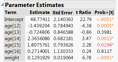
Regression parameter estimates from regression : (I assume the estimates on age groups are what you want to test)
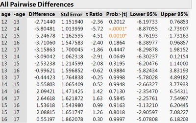
The results from running Multiple Comparisons:
Comparing the pair Age 14 to Age 16: the difference in slope: 2.3656086-0.2714001=2.0942085
- Mark as New
- Bookmark
- Subscribe
- Mute
- Subscribe to RSS Feed
- Get Direct Link
- Report Inappropriate Content
Re: comparison of slopes
Hi hillaryvoet,
If I'm understanding your question correctly, you have a regression with a categorical variable (X1) and continuous variable (X2) and the interaction between them predicting a continuous variable (Y). Your categorical variable (X1) has more than two levels, and you have a statistically significant interaction between X1 and X2 and would like to follow-up on that to see for which groups the regression of Y on to X2 differs. The methods listed by others here don't seem to be testing the pairwise differences in slopes, but rather the pairwise difference in means, assuming a mean level on the continuous regressor (X2). There is a way to get the tests you want, but it'll take a few extra steps. I'll use the Car Physical Data sample dataset for this example.
First I will fit a model like you're working with. I predict Weight on the basis of Country and Turning circle, and their interaction.
In the regression plot we can see directly what you're asking for, three tests of the differences in slopes between each pair, Japan/Other, Japan/USA, Other/USA.
Tests produced under Effect Details for the factor of Country, (for instance LSMeans Differences Student's t), are not tests of slope differences, but are tests of whether the mean weight of cars differ for those countries assuming the mean level of turning circle.
To reveal a test of slopes, we will go to the top-most Red Triangle > Estimates > Indicator Parameterization Estimates
This will show a table of parameter estimates based on an indicator parameterization (as opposed to effects coding, which is what the regular parameter estimates table is based on) which means the LAST level of your categorical factor is used as a reference category, and estimates are differences from that reference category. This will be useful for us.
Notice that we see no estimates with USA. That's because USA is our reference category, so all estimates are differences from what was estimated for the USA. Country[Japan], with the estimate of 256.78, is how much Japan differs from the USA in terms of weight on average. Notice that is the same thing we saw above in the ordered differences report table.
If we look at the interaction parameter estimates we can use the same logic: Country[Japan]*(Turning Circle-38.5862), and the associated estimates, is how the slope for Japan differs from the slope for the USA (by the way, the slope for the USA is listed under "Turning Circle" since it's the reference category, so 155.46 is the USA). Notice that the slope for Japan is nearly the same as the slope for the USA -- different by only a value of 0.06, p = 0.9985. The slope for Other differs from the USA by -42.38, p = 0.2193.
So we're almost there. We're missing one test, Japan vs Other. To get this we need to make JMP treat Japan, or Other, as the reference category, and then rerun this analysis. I'm going to choose to treat Other as the reference category. To change the reference category we'll change the Value Ordering property for the column Country. Right click on the column in the table and go to Column Info. Click on Column Properties, and then select Value Ordering. To change the ordering, select "Other" and click Move Down. The last category listed will be the reference category. Click okay when you're done.
To rerun the model, go to the top-most red triangle of your existing Fit Model output > Script > Redo analysis.
The "Indicator Function Parameterization" now lists the same analyses we saw before, but with "Other" as the reference category.
And now we have our last test, the slope difference between Japan vs Other, which we find in the row "Country[Japan]*(Turning Circle-38.5862)". A difference of 42.45, p = 0.2204.
So we have our three pairwise slope tests.
Japan vs USA, difference = 0.06, p = 0.9985.
Other vs USA, difference = 42.38, p = 0.2193.
Japan vs Other, difference = 42.45, p = 0.2204.
I hope this helps!
- Mark as New
- Bookmark
- Subscribe
- Mute
- Subscribe to RSS Feed
- Get Direct Link
- Report Inappropriate Content
Re: comparison of slopes
Hi Julian,
Thank you for your detailed answer. I really appreciate your going through
the stages of the explanation one by one. One comment and one further
question:
If the categorical variable has more than three levels this means changing
the ordering of the values as many times as necessary to cover all the
pairs of comparisons. This isn't difficult, but it would be nice if JMP
could build this into the menu as a single step.
I didn't understand the difference between the regular parameter estimates
and the indicator function parametrization estimates. Nor do I understand
the role of the constant (38.5862) subtracted from the continuous
predictor (turning circle) in obtaining the estimates. When using SAS and
the ESTIMATE statement in PROC GLM one can get an estimate of the
regression slope for each value of the categorical variable. How can I get
these values in JMP?
Thanks again,
Hillary.
From: Julian Parris
Sent: Wednesday, May 25, 2016 12:44 AM
To: hillaryvoet <hillary.voet@mail.huji.ac.il>
Subject: You have been mentioned by Julian Parris in Re: comparison of
slopes in JMP User
JMP User Community
<https://community.jmp.com/?utm_source=JIVE&utm_medium=email&utm_campaign=System%20Email%20Tracking>
You have been mentioned
by Julian Parris
<https://community.jmp.com/people/julian?et=notification.mention> *in Re:
comparison of slopes in JMP User* - View Julian Parris's reference to you
<https://community.jmp.com/message/228776?et=notification.mention#228776>
- Mark as New
- Bookmark
- Subscribe
- Mute
- Subscribe to RSS Feed
- Get Direct Link
- Report Inappropriate Content
Re: comparison of slopes
Hi Hillary,
You're welcome! It looks you replied to my post via email so I hope the screenshots came through.
Let me tackle your questions first:
- Difference between regular parameter estimates and the indicator parameter estimates: This has to do with how JMP parameterizes categorical variables. There are two ways to do this: effect coding, and indicator coding. Effect coding, common in designed experiments, models the parameters such that the estimates are with respect the grand mean across all groups. So, the regular parameter estimates list a difference from average response. Indicator coding means that estimates reflect a difference from some baseline or reference group. Both types of parameterization are useful at times, but effect coding, the default in JMP, has better properties for more complicated models and is thus prefered.
- The naming of the interaction terms with subtracting a constant: this is called centering, or using a centered polynomial. That constant is the mean of that variable, and in constructing the interaction term the cross product between variables is found my multiplying not the original values of the variable, but the value of the variable after subtracting the mean. This also has desirable properties for complicated models, and has the useful effect of keeping lower order terms in the model more interpretable. In short, the parameter estimates of lower order terms, say of Japan vs USA in terms of weight, indicate how much those countries differ for cars of average turning circle. Without centering of the turning circle variable, that lower order term would indicate the estimate when cars have 0 turning circle radius (which doesn't really make any sense). For more information about centering a polynomial and its consequences, see my response and video on this post: estimates in multipule regression
- There are a few ways to get the slopes for each group. Using the indicator parameterization table you can just look at the estimate for your continuous variable, and that will be the estimate for the slope of the reference category. Another way is using Analyze > Fit Y by X. Set this up with just your continuous Y and continuous X, click okay, then once you have the output go to the Red Triangle > Group by, and then select your categorical variable. Now, whatever action you perform will be done separately for each X. Go back to the Red Triangle > Fit Line. You will now have as many linear fits as you have levels of your categorical X. You can read off the individual slopes there.
As for your comment, I agree! After I posted my response I started thinking about how utterly manual this is! If you have many levels of your categorical X this would be a bit tedious. So, I worked on an add-in to automate this: Compare Simple Slopes in One-Way ANCOVA (w Interaction) add-in
I hope this helps!
- Mark as New
- Bookmark
- Subscribe
- Mute
- Subscribe to RSS Feed
- Get Direct Link
- Report Inappropriate Content
Re: comparison of slopes
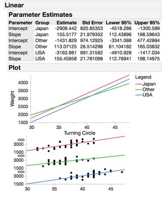
Another option for comparing slopes across groups is the non-linear platform (which has a linear fit option). Using the car data as Julian did if you have weight as the Y, Turning Circle as the X and then Country as the Group and then under the Fit Curve>Polynomials>Fit Linear you will get a linear fit for each group:
Then under the Linear red triangle select "Compare Parameter Estimates" and you will get a comparison of the intercepts and slopes (note they have been estimated for you in the table shown above). This isn't exactly what you were looking for as the comparison of the slopes is done by ANOM so the comparison is to the overall slope: does the slope from any group differ from the overall slope? is the question under consideration with ANOM.
- Mark as New
- Bookmark
- Subscribe
- Mute
- Subscribe to RSS Feed
- Get Direct Link
- Report Inappropriate Content
Re: comparison of slopes
Great suggestion, Karen! That's certainly the most direct way to produce those analyses when a comparison to the overall/mean slope is needed.
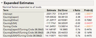
Edit: Another option if we're after comparisons to the average slope (even though I prefer ANOM) is requesting Expanded Estimates from the original Fit Model report (Top Red Triangle > Estimates > Expanded Estimates). Expanded estimates show all parameters for all levels of the nominal factors:
Unlike the Indicator Parameterization estimates these are all with respect to the average response. "Turning Circle" here is then the average/overall slope, and the estimates for the interaction parameters are the differences in slope for each region compared to the average.
Interestingly... some of these estimates are ever so slightly different than the ANOM in the non-linear platform. The given estimate in the ANOM table for the slope of Japan is 155.5, which is indeed equal to what we recover from the expanded estimates report in Fit Model: 141.35+14.16 = 155.51. However, in the ANOM report, the mean slope is listed/drawn at 144.71, which isn't correct. (155.52+113.07+155.46)/3 = 141.35.)
Recommended Articles
- © 2026 JMP Statistical Discovery LLC. All Rights Reserved.
- Terms of Use
- Privacy Statement
- Contact Us

