Equation prediction

[#1]

Dear All, I need a help about prediction from polynomial degree equations. I have a jmp file at the attachment. ı am interesting result change with time(day). Additionally ı want to predict what time Result is equal to 22. For that purpose ı use 

Analyse ---> Fit Y by X

Y, Response: Result

X, Factor: Time(day)

Then

from red triangle I select  Fit,polynomial --> 3,cubic.

The below equation is obtained;

Result = 13,063024 + 1,1850185*Time(day) - 0,3382576*(Time(day)-5,5)^2 + 0,0272922*(Time(day)-5,5)^3

I want to predict what time(day) result will be equal to 22. 

How can I use the above equation. 

Is there anyone can help for this. 

You can see at the attached jmp file.

[#2]

This picture tells a story:

Screen Shot 2017-06-21 at 11.11.52.png

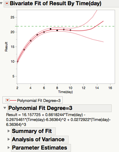
As you know, when building empirical models, extrapolation is always dangerous. To really answer your question, you need more data.

[#3]

Ian's picture leads me to ask the question: is there an asymptote at aboout 22? So I would be asking someone with the subject matter knowledge about the data as I would consider fitting a model such as a logistic model to the data. But as Ian pointed out you don't know what happens beyond time 10 for sure without more data.

Analyze>Specialized Modeling>Nonlinear

Result = Y

Time = X

Click ok

Red triangle>Sigmod curves>logistic curves > Fit Logistic 3P

or copy and run this script:

Fit Curve( Y( :Result ), X( :Name( "Time(day)" ) ), Fit Logistic 3P )

[#4]

You can save the fitted model as a column formula. Click the red triangle next to Polynomial Fit Degree=3 under the plot but above the rest of the outline and select Save Predicted. Now select Graph > Profiler, select your new prediction column, click Y, Prediction Formula, and then click OK. You can now change the predictor value to 22 or any other value by clicking, dragging, or typing. The prediction appears on the response axis.

Ian's warning about extrapolation stands, however.

[#5]

Unless I'm mistaken, it's a predicted value of 22 that is of interest (hence my dotted green line).

[#6 · Accepted solution]

Ian is correct and I missed that point. The desirability function in the Prediction Profiler can help. Click the red triangle next to Prediction Profiler and select Optimization and Desirability > Desirability Functions. The default mapping of desirability to the response is maximize. Ctrl-click (Windows) or Cmd-click (Macintosh) the desirability function plot and change the goal from Maximize to Match Target. Now update the Low, Middle, and High values to represent your goal. (Don't change the Desirability values!) For example, let's say that I want 22 +/- 0.1 for my response. Enter 21.9 for Low, 22 for Middle, and 22.1 for High. Click OK. Now click the red triangle again and select Optimization and Desirability > Maximize Desirability.