- JMP User Community
- :
- Blogs
- :
- JMPer Cable
- :
- Type 1 Gauge Study in JMP 17
- Subscribe to RSS Feed
- Mark as New
- Mark as Read
- Bookmark
- Subscribe
- Printer Friendly Page
- Report Inappropriate Content
Type 1 Gauge Study is new in JMP 17. This type of measurement systems analysis studies the bias and repeatability of a gauge. In other words, can the gauge repeatedly measure a part and obtain measurements that are close to a known reference standard?
Type 1 Gauge Studies should be your first step in assessing your measurement system. Performing a measurement systems analysis with a gauge that cannot precisely and repeatably measure your parts is an exercise in futility. You must first determine if you have a good gauge before looking for other sources of measurement variation.
Example
First, open the Type 1 Gauge MSA data table in the variability data folder.
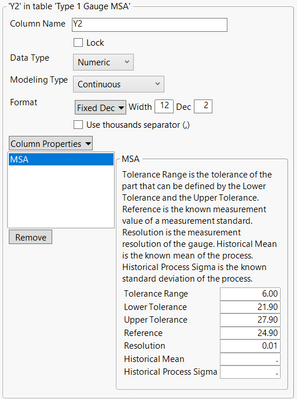
dt=Open("$SAMPLE_DATA/Variability Data/Type 1 Gauge MSA.jmp");The data found in column Y2 are repeated measurements for a part. It is important to note that the measurements use one operator and one reference part. Y2 has a Measurement Systems Analysis (MSA) column property.
The tolerance range (6) is the tolerance of the part that can be defined by Upper Tolerance (27.9) to Lower Tolerance (21.9). The industry typically sets these values. Reference (24.90) is the known measurement value of a measurement standard. You may have a “master sample” that provides this information, and it may be defined by law, etc. Resolution (0.01) is the measurement resolution of the gauge. This value is typically stated in the manufacturer’s specification of the gauge. The Historical Mean (missing) is the known mean of the process. Historical Process Sigma (missing) is the known standard deviation of the process. Historical Mean and Historical Process Sigma are not used in the Type 1 Gauge analysis but are used in other types of analyses such as Gauge R&R.
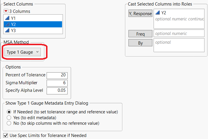
Type 1 Gauge is found in the Measurement Systems Analysis platform. Select Analyze->Quality and Process->Measurement Systems Analysis. Set the MSA Method to Type 1 Gauge. Specify Y2 as Y, Response.
Notice in the Options section of the dialog that you can define the Percent of Tolerance. This value specifies the percent of part tolerance used to compare against the measurement variation. The default value is 20%. Sigma multiplier specifies the constant multiplied by sigma (6 for a 6 sigma process). The alpha level allows you to specify the alpha used for the bias test (default 0.05).
The Show MSA Metadata Entry Dialog specifies whether the MSA Metadata dialog is shown after you click OK. This dialog lets you load the metadata from a data table or manually enter the metadata for each column. A tolerance range/upper and lower tolerance, as well as a reference value, are necessary for a Type 1 Gauge Study.
Click OK to see the report for Y2.
Run Chart
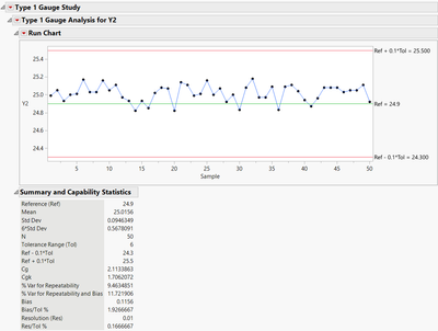
We can see from the Run Chart that the observed measurements are close to the reference standard (green line), and all measurements are within the percent of tolerance*tolerance range (red lines). Points outside the Run Chart limits indicate that the measurement variation was too large in relation to the parts tolerance. In other words, the gauge is too variable. Note that most observations fall above the reference standard (green line), which indicates possible bias in the measurements.
Summary Statistics
Reference, Tolerance Range, and Resolution came from the MSA column property for Y2. Mean, Std Dev, 6*Std Dev, and N are calculated the same as in the Distribution platform. There may be some statistics you are not familiar with, so I have included terms, descriptions, and equations in the following table.
| Statistic | Description | Formula |
| % Var for Repeatability | Variance percentage associated with repeatability |  |
| % Var for Repeatability and Bias | Variance percentage associated with repeatability and Bias |  |
| Cg | Ratio between precision and tolerance (potential capability) |  |
| Cgk | Ratio between the accuracy and the tolerance (actual capability) |  |
Values greater than 1.33 for Cg indicate that the spread of the gauge’s measurements is adequately narrow in relation to the tolerance range. A Cgk value greater than 1.33 denotes a capable gauge.
Bias Test
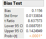
As we noted in the run chart section of this blog, most of the points fall above the reference line (green line). Bias is the difference between the mean and reference value. A t-test is often used to determine if there is bias or not. Click the red triangle next to Type 1 Gauge Analysis for Y2 and select Bias Test.
Histogram
A histogram provides a graphical representation of bias and precision. Click the red triangle next to Type 1 Gauge Analysis for Y2 and select Histogram.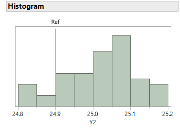
Conclusions
Although the Cg and Cgk values are greater than 1.33, indicating a capable gauge, the gauge provides biased measurements of Y2, as evidenced by the bias test. Further MSA analysis should only be performed once we are satisfied with the capability of the gauge.
You must be a registered user to add a comment. If you've already registered, sign in. Otherwise, register and sign in.
- © 2025 JMP Statistical Discovery LLC. All Rights Reserved.
- Terms of Use
- Privacy Statement
- Contact Us

