New in JMP® 18: Python jmp.DataTable and pandas.DataFrame

[#1]

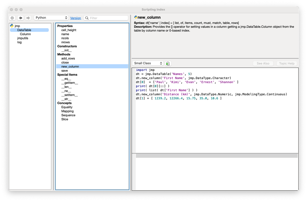
JMP 18 brings powerful new capabilities in its Python integration, including: 

• An embedded version of Python 3.11.
• Package installation support.
• Python-aware script editor that can run pure Python scripts.
• An import jmp package providing Python access to JMP functionality.
• Enhanced error reporting.
• Scripting index support documenting and providing examples for the new functionality under a Python category.

Today, I'm focusing on the jmp.DataTable object and the changes JMP 18 has made with respect to Python Send ( dt ) and Python Get( df ), where "dt" is a data table and "df" is a pandas.DataFrame.

Beginning with JMP 14 and up until JMP 17, users could transfer a copy of a JMP data table to the Python environment using the JSL command Python Send( dt );. It functioned behind the scenes with JMP writing the data table to a temporary CSV file in the file system and then invoking pandas to read the CSV file from disk into a DataFrame.

While that worked just fine for small files, it wasn't suitable for larger data. The first issue is that it required using the file system for data transfer. The second problem is a loss of precision when going from binary to text and then back to binary.  Third, the CSV file is often dramatically larger than the original binary data. Finally, the data in Python is merely a copy, without any way to manipulate the original table. Bringing Python processed data back into JMP using Python Get ( df ); follows exactly the same process in reverse. Python Get( df ); was left intact for compatibility reasons.

But now with the advent of JMP 18, Python Get ( dt ); retrieves the data table reference to JSL of the actual table, which is is a zero-copy operation. By necessity, Python Send( dt ); no longer creates a pandas.DataFrame. In Python, you get a jmp.DataTable object, which is a live reference to the JMP data table. This too is a zero-copy operation, allowing direct access from Python to access, edit, and modify the JMP data table. You can create a jmp.DataTable object from Python while creating a new JMP table.

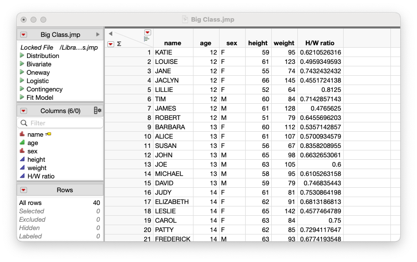
Below is a JSL script using the JMP 18.0 features to take a JMP data table and add a column that is the ratio of two columns from Python. It is performed live on the current data table:

// BigClass_hw_ratio.jsl
// Description: Show JMP 18 Python integration features
// 
Names Default to Here(1);

dt = Open("$SAMPLE_DATA/Big Class.jmp");

Python Send(dt);

Python Submit("\[
import jmp

# print some information on data table properites
print(dt.__class__)
print(dt.name)
print(f'nrows: {dt.nrows}')
print(f'ncols: {dt.ncols}')

# data table object columns may be indexed either by
# column name or index.  Note: slice is only supported
# when using indexes.  Slice on both columns and rows is supported.
for x in dt[0:]:
    print( x.name )
    
# As is Python convention, indexing is 0-based
print( dt['name'][0] )

# create a new column based on data from the original data.
# Because JMP is column centric, the access to
#    jmp.DataTable object is [column][row]
dt.new_column('H/W ratio', jmp.DataType.Numeric)
for idx in range(dt.nrows):
    dt['H/W ratio'][idx] = dt['height'][idx] / dt['weight'][idx]
]\");

It results in this log output:

/*:

<class 'jmp.DataTable'>


Big Class


nrows: 40


ncols: 5


name


age


sex


height


weight


KATIE


0

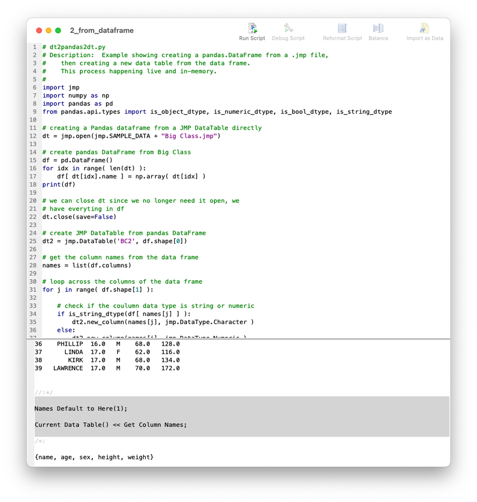
Next, let's see how to work directly from Python. Below is a Python script that:

• Opens Big Class.jmp.
• Creates a pandas data frame in-memory from the jmp.DataTable object.
• Closes Big Class.
• Builds a new JMP data table from the DataFrame.
• Prints the column names of the current data table in JSL.  

The current table is the one just created in Python.

# dt2pandas2dt.py
# Description:  Example showing creating a pandas.DataFrame from a .jmp file,
#    then creating a new data table from the data frame.
#    This process happening live and in-memory.
# 
import jmp
import numpy as np
import pandas as pd
from pandas.api.types import is_object_dtype, is_numeric_dtype, is_bool_dtype, is_string_dtype

# creating a Pandas dataframe from a JMP DataTable directly
dt = jmp.open(jmp.SAMPLE_DATA + "Big Class.jmp")

# create pandas DataFrame from Big Class
df = pd.DataFrame()
for idx in range( len(dt) ):
    df[ dt[idx].name ] = np.array( dt[idx] )
print(df)

# we can close dt since we no longer need it open, we
# have everyting in df
dt.close(save=False)

# create JMP DataTable from pandas DataFrame
dt2 = jmp.DataTable('BC2', df.shape[0])

# get the column names from the data frame
names = list(df.columns)

# loop across the columns of the data frame
for j in range( df.shape[1] ):
    # check if the coulumn data type is string or numeric
    if is_string_dtype(df[ names[j] ] ):
        dt2.new_column(names[j], jmp.DataType.Character )
    else:
        dt2.new_column(names[j], jmp.DataType.Numeric )
	
    # populate the JMP column with data
    dt2[j] = list(df.iloc[:,j])

# Just as JSL has a Python Submit(); to execute Python code
# the jmp object has a run_jsl() command to execute JSL from Python
jmp.run_jsl('''
Names Default to Here(1);

Current Data Table() << Get Column Names;
''')

The following log output is the result:

/*:

         name   age sex  height  weight
0       KATIE  12.0   F    59.0    95.0
1      LOUISE  12.0   F    61.0   123.0
2        JANE  12.0   F    55.0    74.0
3      JACLYN  12.0   F    66.0   145.0
4      LILLIE  12.0   F    52.0    64.0
5         TIM  12.0   M    60.0    84.0
6       JAMES  12.0   M    61.0   128.0
7      ROBERT  12.0   M    51.0    79.0
8     BARBARA  13.0   F    60.0   112.0
9       ALICE  13.0   F    61.0   107.0
10      SUSAN  13.0   F    56.0    67.0
11       JOHN  13.0   M    65.0    98.0
12        JOE  13.0   M    63.0   105.0
13    MICHAEL  13.0   M    58.0    95.0
14      DAVID  13.0   M    59.0    79.0
15       JUDY  14.0   F    61.0    81.0
16  ELIZABETH  14.0   F    62.0    91.0
17     LESLIE  14.0   F    65.0   142.0
18      CAROL  14.0   F    63.0    84.0
19      PATTY  14.0   F    62.0    85.0
20  FREDERICK  14.0   M    63.0    93.0
21     ALFRED  14.0   M    64.0    99.0
22      HENRY  14.0   M    65.0   119.0
23      LEWIS  14.0   M    64.0    92.0
24     EDWARD  14.0   M    68.0   112.0
25      CHRIS  14.0   M    64.0    99.0
26    JEFFREY  14.0   M    69.0   113.0
27       MARY  15.0   F    62.0    92.0
28        AMY  15.0   F    64.0   112.0
29     ROBERT  15.0   M    67.0   128.0
30    WILLIAM  15.0   M    65.0   111.0
31       CLAY  15.0   M    66.0   105.0
32       MARK  15.0   M    62.0   104.0
33      DANNY  15.0   M    66.0   106.0
34     MARTHA  16.0   F    65.0   112.0
35     MARION  16.0   F    60.0   115.0
36    PHILLIP  16.0   M    68.0   128.0
37      LINDA  17.0   F    62.0   116.0
38       KIRK  17.0   M    68.0   134.0
39   LAWRENCE  17.0   M    70.0   172.0


//:*/

Names Default to Here(1);

Current Data Table() << Get Column Names;

/*:

{name, age, sex, height, weight}

Keep an eye out for more samples in future blog posts.