New Control Chart Builder Features in JMP 17

[#1]

JMP 17 brings many new features to Control Chart Builder (CCB), including

• Reorganization of the Quality and Process menu
• Laney P’ and U’ control charts
• Button to switch XBar charts to IMR charts/Label role
• N Subgroups in the saved limits table
• K-Sigma option
• Three Way control chart dialog overhaul
• Connect thru Missing
• Row legend

Reorganization of the menu

The first thing you will notice about CCB is that the quality and process menu has been reorganized.

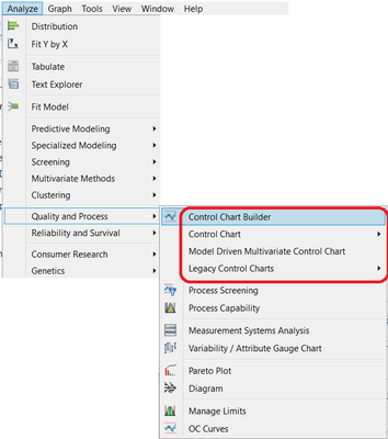Figure 1

All control chart options have been grouped together to appear in the top section of the menu. 

Laney P’ and U’ Charts

Laney P’ and U’ charts are new for version 17. For an example, open Electrical Component Defect Screening found in the Quality Control folder:

Open("$SAMPLE_DATA/Quality Control/Electrical Component Defect Screening.jmp");

To create a Laney P’ chart, click Analyze->Quality and Process->Control Chart->Laney P’ Control Chart. Specify N Defective as Y, n Defective. Specify Week as Subgroup. Specify N Units as n Trials. Click OK.

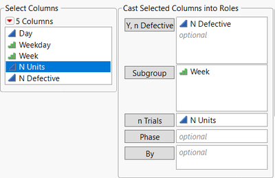Figure 2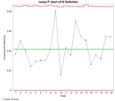Figure 3

To learn more about Laney charts, read my earlier blog post.

Switch to IMR Chart/Label role

Data can sometimes be in a format where the subgroup levels are not unique, but they should be treated as unique.  For an example, open Big Class.jmp found in the sample data folder:

Open("$SAMPLE_DATA/Big Class.jmp");

You want to create a control chart for height using name as the subgroup. Select Analyze->Quality and Process->Control Chart Builder. Drag name to Subgroup and height to Y. An XBar and R chart is created because there are two values for Robert. These two Roberts are not the same person. One Robert is 12, and the other Robert is 15. These values of height should be treated as unique values. You can do this by clicking the “Switch to IMR Chart” button at the bottom of the control panel.

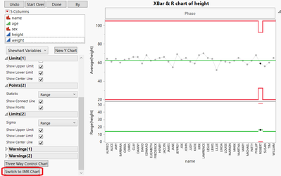Figure 4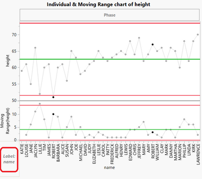Figure 5

The chart changes to an IMR chart.  Each height value for Robert is treated as a separate subgroup. The x-axis maintains data table row order rather than alphabetical order. This is accomplished by placing name into the Label role rather than the Subgroup role. Instead of using the Switch to IMR Chart button, we could have created this chart by dragging height to Y and name to the Label role in the bottom left of the control chart. The label role is useful when the x-axis variable is not unique but should be treated as unique.

N Subgroups in the saved limits table

The number of subgroups is now saved to limits tables. Click the red triangle next to Control Chart Builder and select Save Limits->in New Table. A new row for _N Subgroups contains the number of subgroups.

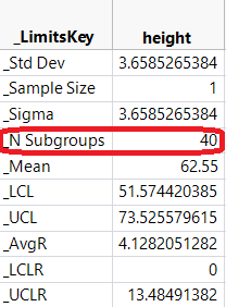Figure 6

K Sigma

A K Sigma option has been added. By default, K Sigma is 3. Suppose, for the example, above (Switch to IMR Chart/Label role), you wanted to use a K Sigma of 4. Click the red triangle next to Control Chart Builder and choose K Sigma. Enter 4 and click OK.

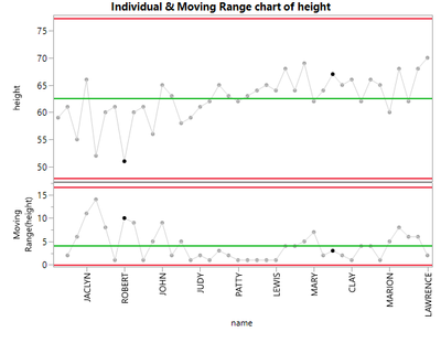Figure 7

 Notice the limits are now wider (compare to Figure 5 above).

Three Way Control Chart dialog

The Three Way Control Chart dialog has been updated so that you can define more options prior to creating a chart.

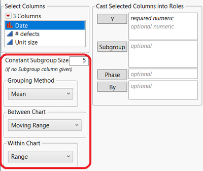Figure 8

Constant Subgroup Size is new and allows you to define a constant for the subgroup size. There are now three drop boxes available. The first drop box allows you to select the Grouping Method (Mean or Standard Deviation). The second drop box enables you to choose the Between Chart (Moving Range or Median Moving Range). The final drop box lets you define the Within Chart (Range or Standard Deviation).

Connect Thru Missing

A Connect Thru Missing option now allows you to connect observations when there are missing data points. For an example, run the following:

dt=Open("$SAMPLE_DATA/Quality Control/Pickles.jmp");
Column(dt, "Acid")[3]=.;
obj=dt<<Run Script("Individual Measurement Chart");

Notice the gap in the connect line between samples 2 and 4. Click the red triangle next to Control Chart Builder and select Connect Thru Missing.

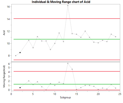Figure 9

Sample 2 is now connected to sample 4.

Row Legend

It is now possible to add a row legend to CCB. In the example above (Connect Thru Missing), right-click in the graph and select Row Legend. Choose Time from the Columns panel. Choose Alphanumeric for Markers. By default, you will have labels A, B, and C, but you can change these to X, Y, and Z to match what is found in the Time Marker column in the Pickles data table.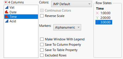Figure 10

 Clicking OK results in the following:

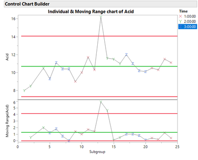Figure 11Note: The row legend option is only available when there is one row per subgroup.

Conclusion

JMP 17 offers many new features in CCB that give users more flexibility in monitoring their processes.