A bioassay is an analytical method to determine concentration or potency of a substance by its effect on living cells or tissues. Bioassays are used to estimate the potency of agents by observing their effects on living animals (in vivo) or tissues (in vitro).
Analysis of biological assays and tests is commonly carried out in the pharmaceutical and biotechnology industries. It is an important component to regulatory submissions, development of standard operating procedures and maintenance of good manufacturing practices.
Different methodologies are used in Bioassay tests. In this blog I describe bioassays examples using JMP that are commonly used.
The Parallelism Test
The Parallelism Test provides an analysis for testing if the fitted models between groups have the same shape but are shifted along the X axis. According to the United States Pharmacopeial Convention (USP) standards, parallelism between a pair of doses – responses functions need to be achieved prior to validating a potency bioassay. The parallelism test is found in the Fit Curve platform for Sigmoid Curves. In this example, a modified version of the Bioassay data set from the JMP data sample library was used. A logistic 4 Parameters model was fit to the three different formulations. Those three curves were analyzed and tested for parallelism (Figure 1). Notice that the horizontal shift is the same at all doses. Two curves that only differ by a horizontal shift are said to be parallel. If the test item did not have the same biologically active component as the standard, the relative potency would vary over the dose range. In this example, all curves have the same shape but are shifted horizontally, and a high P-value validates our findings, concluding that the curves from the three formulation curves are parallel.
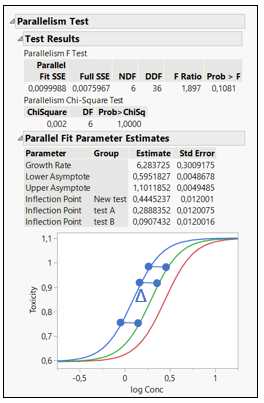
Figure 1: Parallelism Test (Notice that the Log (Relative Potency) horizontal shift ∆ is the same at all doses)
The Relative Potency
How is Relative Potency estimated from EC50? EC50 is the dose required for an individual to experience 50% of the maximum effect (Figure 2). Relative Potency estimates are generally calculated as a simple ratio: the EC50 of a well- characterized standard divided by the EC50 of a sample. Such estimates are valid only when the dose–response curves for the sample and standard are parallel and exhibit the same maximum achievable response (efficacy).
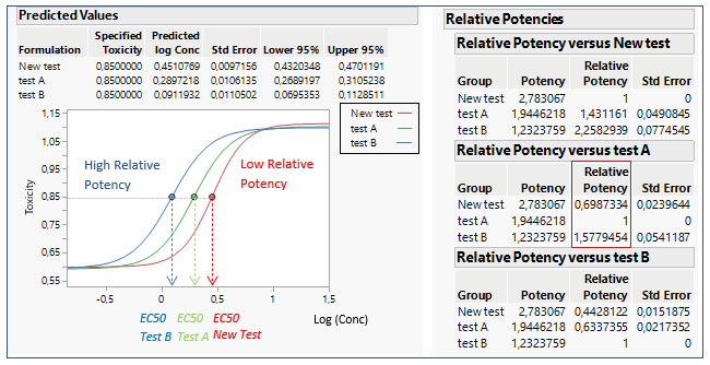
Figure 2: EC50 representations and calculations for 3 formulations
The Relative Potency in JMP is found below the parallelism test. In figure 2, three different formulations are compared: Test A, Test B and New Test.
When comparing the New Test versus Test A, the relative potency for the New Test is smaller than one. This indicates that their potencies are different, and the New Test is less potent than Test A, as we can see on the graph. The relative potency for Test B is greater than for Test A. This means that drug formulation B increases in toxicity as a function of concentration faster than Test A. If Relative Potencies are nearly one, this indicates that their potencies are similar.
The Equivalence Test
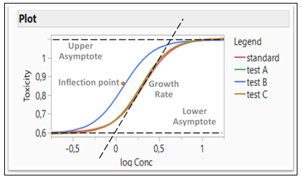
Figure 3: Logistic 4P model fitting four formulations (Four Parameters: Growth Rate, Inflection Point, Lower and Upper Asymptote)
In the Fit Curve platform, the Equivalence Test option gives an analysis for testing the equivalence of models across levels of the grouping variable. The Bioassay data is used for this example (Figure 3). Four different formulations are compared and tested whether they are equivalent. A Logistic 4P shows a fit for four Parameters (Growth Rate, Inflection Point, Lower and Upper Asymptote). Those four parameters are tested whether they are equivalent or not. Note that Test B in blue is different than all three other formulations
After selecting the option for Equivalence Test, you specify the level of the grouping variable that you want to test against every other level (Standard formulation is used as the grouping variable or reference). A report is displayed for every level versus the chosen level. Figure 4 shows an example of two comparisons (Test A versus Standard and Test B versus Standard).
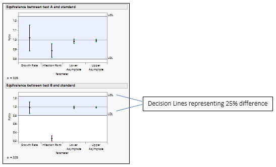
Figure 4: Equivalence Test for Test A versus the Standard and Test B versus the Standard.
The equality of the parameters is tested by analyzing the ratio of the parameters. The default decision lines are placed at ratio values of 0.8 and 1.25, representing a 25% difference.
If all the confidence intervals are inside the decision lines, then the two groups are practically equal. If a single interval falls outside the lines, then we cannot conclude that the groups are equal. In our example, Test B is not equivalent to the Standard, as the inflection point for drug formulation B is lower than the standard, which agrees with the Figure 3.
The Inverse Prediction and EC50
You might be interested to know at which Dose or Concentration of the drug reaches a specific Toxicity value. This is to predict the X values for a specific Y value or what inverse prediction does.
This is an important step for example to calculate EC50/IC50. The EC50 is the concentration of a drug that is necessary to cause half of the maximum. In a binding experiment, the IC50 is the concentration of a ligand or inhibitor at which half of the target is present at the bound stage. It is commonly used a measure of a drug’s potency (see above), although the use of EC50 is preferred over that of “potency”, which has been criticized for its vagueness (ref).
From the fitted curve, use in the red triangle of model the option custom inverse prediction, specify the Y (the response like toxicity) to predict the X (like log concentration or dose). A graph and the predicted value of the X with 95% confidence intervals are displayed (Figure 5).
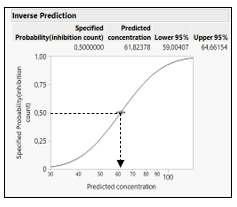
Figure 5: Inverse prediction estimation
The Vmax and Km Estimation from Michaelis-Menten Kinetics
In biochemistry, Michaelis-Menten kinetics is one of the best-known models of enzyme kinetics. It is named after German biochemist Leonor Michaelis and Canadian physician Maud Menten. The model takes the form of an equation describing the rate of enzymatic reactions (v), its formula and the curve is shown in Figure 6.
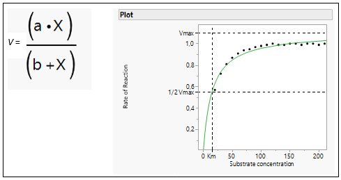
Figure 6: Michaelis Menten Equation and model fit.
The parameter a represents the maximum reaction rate (in literature often referred to as Vmax), and the b parameter (in literature often referred to as the Michaelis Constant or Km) is the value of x such that the response is half Vmax. It is an inverse measure of the substrate’s affinity for the enzyme. Km is a measure of the affinity of the enzyme for the substrate. Substrates that bind tightly have small Km values; substrates that bind weakly have large Km values.
Using the Fit curve platform and choosing the Michaelis-Menten model, is easy to extract both Vmax and Km from the equation. See the example in Figure 7.
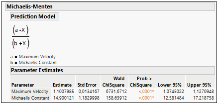
Figure 7: Parameter a (Vmax) and Parameter b (Km) estimation in Michaelis-Menten curve fit.