- New to JMP? Let the Data Analysis Director guide you through selecting an analysis task, an analysis goal, and a data type. Available now in the JMP Marketplace!
- See how to install JMP Marketplace extensions to customize and enhance JMP.
JMPer Cable
A technical blog for JMP users of all levels, full of how-to's, tips and tricks, and detailed information on JMP features- JMP User Community
- :
- Blogs
- :
- JMPer Cable
- :
- How to do a test for curvature in a DOE with JMP
- Subscribe to RSS Feed
- Mark as New
- Mark as Read
- Bookmark
- Subscribe
- Printer Friendly Page
- Report Inappropriate Content
The Engineering Mailbag
Episode 6: Watch out for the curves!
TL;DR: How do you do a simple test for curvature when you put center points in a DOE? Watch the video to find out! Also there's now an add-in to do this analysis - link and details are at the bottom of the article.
As a new feature - I'm going to be providing a quick video walk through with these posts on the key points from the article. Just in case you need to get to the answer quickly.
Introduction

Today's particular question is something that needs to be addressed. It's one I get quite often when talking with people who were trained in classical DOE methods. So, this is an opportunity for me to help out a colleague from Europe and show everyone else something interesting that you might not know how to do in JMP.
The question
Hi, Mike,
I still have a question… If I do centre point runs, I am doing it to check if there is a quadratic term, but I may not be sure which term is quadratic. I should be able to check if there is significant curvature without associating it with any one factor, or am I wrong?
Kevin
My response
Hi, Kevin!
… I did a bunch of research on this curvature test. It turns out that it’s just a t-test! I found the equations in Montgomery’s books. More importantly, it’s really easy to do. It’s not a one-click solution, but I actually like it better, because it forces you to understand the hypothesis. I’ve attached a data table.
- Create a column in your data table that indicates where a row is a corner or center point. This could be done using recode if you have a column with the design code in it.
- Go to Fit Y by X. Put your Response into Y, Response and the column you created indicating corner or center point into X, Factors.
- Click OK.
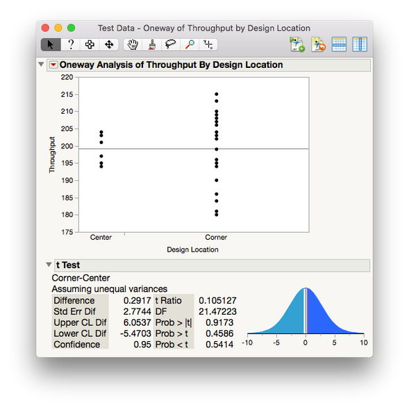
- Under the red triangle, run a t-test (not the pooled one, unless you have replicates). You want the p-value for Prob > |t|. The null hypothesis in this case is that the difference in the means (between center points and corner points) is zero. Montgomery’s explanation is that if the t-test indicates the means are different, then the center points lie on a different plane than the linear elements of the model (there’s curvature).
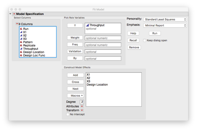
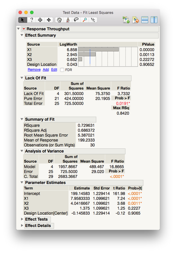
If you want everything in one report (à la [a software package which shall remain nameless but rhymes with “really drab”]), you just have to include the column that flags the center points in the model as a main effect (see screenshot). When you click Run, the Effects Summary at the top would lead you to a similar conclusion (that differentiating between center-points and corner points isn't significant). Have a look and see if you can confirm on your data set.
Best,
M
What the heck did I just suggest?
Before I go down the rabbit hole on this topic, let me give a bit of background on this question – because my colleagues and I get it all the time. Basically, the issue stems from classical screening designs (Fractional Factorial, Plackett-Burman, etc.). These designs generally employ a two-level with multiple center point strategy. The upshot of this is that, within the confines of classical design (more on that later), it’s really efficient resourcewise. The downside is that it only lets you look for main effects and some interactions (if you’re lucky). The center points are added as a hedge to tell the experimenter if they need to consider quadratic terms in later rounds of experimentation. And that’s why you need this test for curvature business.
OK, back to my suggestion. I made what might seem like an odd suggestion. I’m proposing that it’s possible to locate curvilinear ($10 word!) behavior in a designed experiment simply by using the lowly t-test. I mean, it seems like we should need something sexier when looking for a sexily named phenomenon like curvilinear behavior. Well, we don’t. And it turns out, this is not my idea. As I mentioned, the first example that I found of the technique is in Douglas Montgomery’s book, “Design and Analysis of Experiments.” This book was required reading in my first stats class in grad school. Good class, great book. Anyway, back to the topic at hand.
I’m not going to go into all the math of why this works, but here’s the basic idea: If the data collected from a system under study has strictly linear relationships, (e.g., you can connect all points in the data set using just straight lines), then the confidence interval for the mean of data set (excluding the center points) should contain the confidence interval of the mean of the center points. Therefore, if we do a t-test on the means of the edge and corner points vs. the global center points, low p-values would be evidence of curvature somewhere in the system and high p-values would indicate insufficient evidence for curvature in the system. That doesn’t mean it’s not there, just that things are too noisy to tell. Now, since that’s a lot to take in, let’s have a look at some examples so you can see what this looks like.
A trivial example
This is probably easiest to visualize in a trivial case with two continuous factors. Note here that I’m simulating the data and am running with a lot more data than you normally would with a two-factor design. This is for illustrative purposes, so just go with me. Also, note that all the examples in this post are on JMP Public, so you can get the data sets there if you want to play with them.
OK, here’s a designed experiment with two factors and three center points.
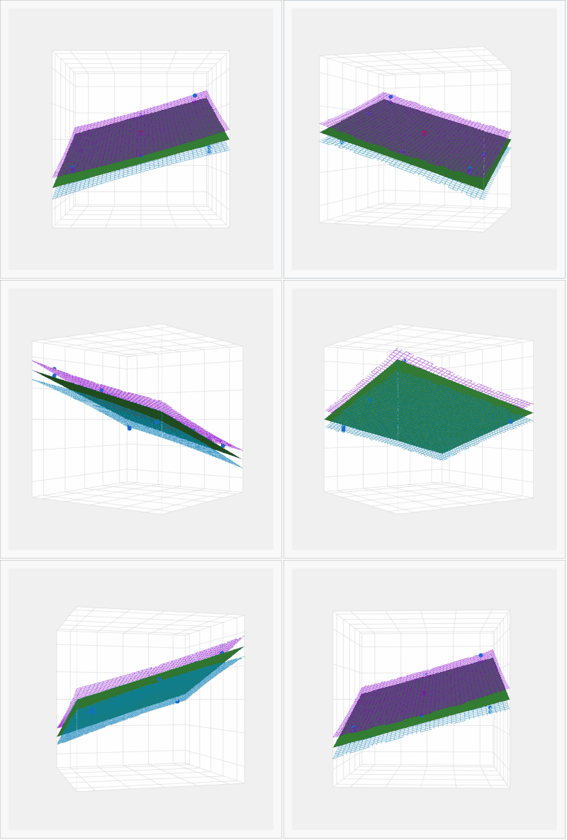
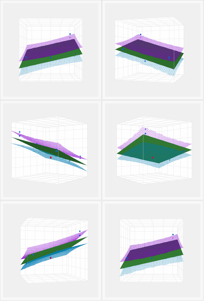
The center points are colored red so that they can be located later. Now, let’s simulate some data into the design without any quadratic effects. In JMP, we can do this using the simulate response capabilities in the DOE platforms. Now, before we look at that t-tests, let’s have a look at what’s going on in the data itself. We’ll turn to a 3D scatterplot. I’ve added the fitted model with 95% confidence interval to show the plane that Montgomery mentions.
You can see that when there is no curvature present, the data points sit within the region defined by the upper and lower confidence intervals (blue and purple meshes).
Now, let’s do one where I’ve put some curvature into the simulated model. I’m using the same linear and two-factor interaction coefficients and just added in some quadratic effects to the data. First, let’s have a look at the 3D plots:
Notice how the red center points are no longer in the plane defined by the blue edge/corner points? Do you also see how the center points are outside the confidence interval for the surface?
Now if we look at the t-tests for these data sets (I used a column switcher in JMP Public to show both), we can see that the confidence intervals for the center points and edge locations overlap nicely in the case where there is no curvature. The p-values for that t-test are quite high, just like we would expect. Then you can switch to the case where there is curvature and see the differences in the confidence intervals and the p-values.
The t-test indicates that there is strong evidence that the center points are not in the same population as the edge/corner points. However, we know that the data is collected from the same system, so there has to be another explanation – which is that the system is more complex that we thought and has curvilinear behavior.
Something a little more complex
Next, let’s turn up the heat on the problem a bit: five factors. The question here is, does the same logic hold for multiple factors as for two? We can’t really visualize this, so we’re going to have to rely on the p-values from the t-test. But we’re asking the same question: does the confidence interval from mean for the center points overlap with the mean from the edge/corner data points? That’s it. And, the same logic still holds.
In this example, I’ve done basically the same thing as in the first one. Below is the scatterplot matrix for the design space. Red marks are center points, blue ones are edge or corners. Also note that some of the data points are missing from a classic full factorial design. I did that to show that this works even with the JMP custom design methodology.
And if we look at the t-tests for the two simulations, we can see the p-values indicate really clearly when there is curvature present in the data set.
And that would appear to be that. Right?
Well, not really. You see there’s another school of thought around DOEs, and I’m going to argue that it solves this problem more efficiently than just slapping some global center points on a screening design and calling it a day.
What modern DOE says you should do about curvature
This whole issue of curvature in a DOE stems from two problems in classical design. The first is the fact that, at one point, people had to do the calculations for DOEs on an actual pad of paper with an actual pencil and probably an RPN calculator (for true geek cred). The designs were therefore chosen to make these calculations as easy as possible. This imposed the idea of orthogonality into the world of experimental design. Orthogonality makes the math a lot easier for people to wrap our heads around. The second problem was the actual creation of the design. Orthogonal designs are fairly easy to conceptualize and fit nicely with the traditional scientific method. They could be easily codified into experimenters’ reference books.
Both of those problems are now solved. Odds are pretty good that you’re not doing data analysis with a calculator (RPN or otherwise). And, you’re probably not consulting some dusty tome to determine your experimental set up, although you might be using the digital equivalent and not know it. The fact is that, unless you’re in a stats class with a really hardcore prof, you’re going to use software to analyze your design and probably generate it, too. This means that you don’t have to do DOE analysis with a pencil and paper – you can let the computer figure it out. It also means that you can let computer algorithms figure out where experiments should go in the design space, allowing you to create a custom design to your exact specifications. Throwing the old requirements out the window gives you access to an incredibly powerful class of tools called modern experimental designs.
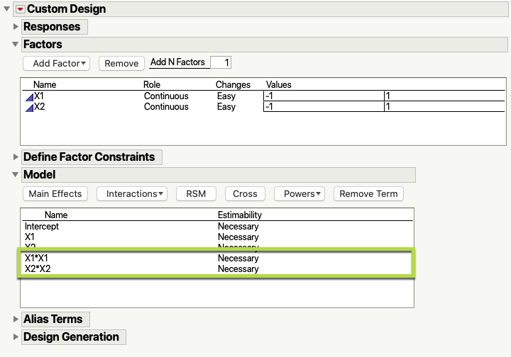
I’m not going to go too far into modern DOEs (there are great books out there on the topic: this one and this one are good places to start) and new articles are coming out all the time in the literature. I am going to focus in a little on one part of modern DOE: the optimal design. The nickel tour version of optimal design is that it allows you to define where you think the curvature is from the beginning. The algorithm then sets up the appropriate experimental conditions to test if it’s there without wasting anything. And that’s important. It’s pretty rare to run into a situation where you don’t have some idea if there’s curvature in the system of study. If you’re working with subject matter experts during the design generation process, they should know that kind of thing. Here’s a snapshot of what that looks like in JMP:
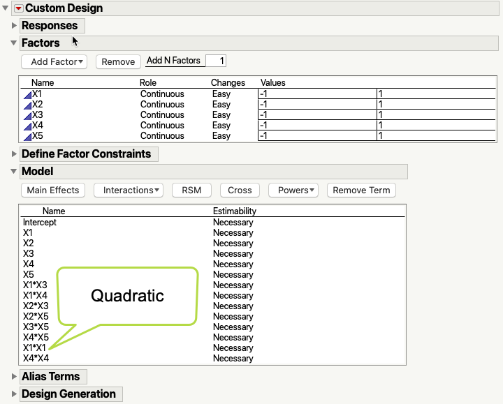
In the model section, I’ve indicated that I think main effects are important and that the interaction is important. The green box around the two squared terms indicates that I think there is curvature in the system in those two factors. The optimal design will then put the center points in the correct places to test for that. Now, if I had five factors, I could choose which ones I want to explore for curvature by including only them in the model terms, like this:
Note all the combinations I’m not including here (interactions and powers); they are all material that I don’t have to use. And when we analyze this design, we’ll still be able to check for curvature as part of the model generation process:
Now, if you want to check for curvature as part of a screening design, you also have a modern method: definitive screening designs. They have center points baked in and are still much more efficient that fractional factorial and other design types. There are some great resources by Brad Jones on the JMP Community. Here are some of my favorites:
- Introducing Definitive Screening Designs
- 21st Century Screening Designs
- Proper and improper use of Definitive Screening Designs
- Powerful Analysis of Definitive Screening Designs
- Simulating Responses and Fitting Definitive Screening Designs
Final thoughts
So, that’s it. It’s a great idea to watch out for curves in your designed experiments. And you can easily test for curvature with center points in JMP using a t-test. There’s nothing magical about the analysis, but it can be tricky to interpret. My colleague @Ross_Metusalem created an add-in that does an excellent job of doing this analysis and presenting the results for you. Have a look here: Pure Quadratic Curvature Test. Until next time, TTFN!
You must be a registered user to add a comment. If you've already registered, sign in. Otherwise, register and sign in.
- © 2026 JMP Statistical Discovery LLC. All Rights Reserved.
- Terms of Use
- Privacy Statement
- Contact Us

