JMPer Cable
A technical blog for JMP users of all levels, full of how-to's, tips and tricks, and detailed information on JMP features- JMP User Community
- :
- Blogs
- :
- JMPer Cable
- :
- Genetic Association with JMP Genomics, Part 3c: Q-K Mixed Model
- Subscribe to RSS Feed
- Mark as New
- Mark as Read
- Bookmark
- Subscribe
- Printer Friendly Page
- Report Inappropriate Content
Q-K association analysis was developed to perform association mapping while controlling for population structure and/or familial relatedness. The “Q-K” in this name refers to the two kinds of information that get included in the model. The Q matrix contains information about population structure (See Part 3b: Population Structure Matrix). The K matrix contains more fine-grained information about relatedness, usually IBD measures calculated from the marker data (See Part 3a: Marker Based Relationship Matrix).
As in other kinds of association mapping, in Q-K association analysis an individual statistical model is created for each marker, using the trait as a dependent variable and the marker as an independent variable. The variables that constitute the Q and K matrices are also included in these models: Q variables as fixed effects, and K variables as random effects. Either the Q or the K variables may be omitted from the models, as desired.
To run Q-K association analysis in JMP Genomics, three things are needed: a data file containing the traits to be analyzed, the marker genotypes, and the Q and K variables to be used in the analysis. An annotation data set is optional.
- Use the File > Open command to open the PCA results merged file, called pca_output_pcm.sas7bdat
- Also Open the file with the “square root” of the IBD matrix from the Relationship Matrix procedure, called rice_genos_recgeno_rm.sas7bdat.
- Note that this file should be replaced with the compressed K matrix file, rice_genos_recgeno_ibd_kc.sas7bdat, if applicable.
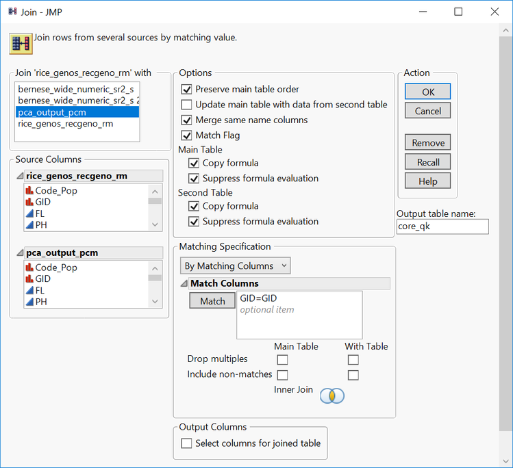
- With the file rice_genos_recgeno_ibd_kc.sas7bdat in the foreground, select Tables > Join.
- In the top left box, select the file pca_output_pcm.sas7bdat
- Check the box labeled Merge same name columns
- Select the variable GID in the two Source Columns boxes, and then click the Match
- Assign the Output table name as core_qk.
- Click OK to create the new joined file.
- When the new data file appears, select File > Save As…
- Change the Save as type option to SAS Data Set and click Save
- From the Genomics Starter menu, choose Genetics > Other Association Testing > Q-K Mixed Model.
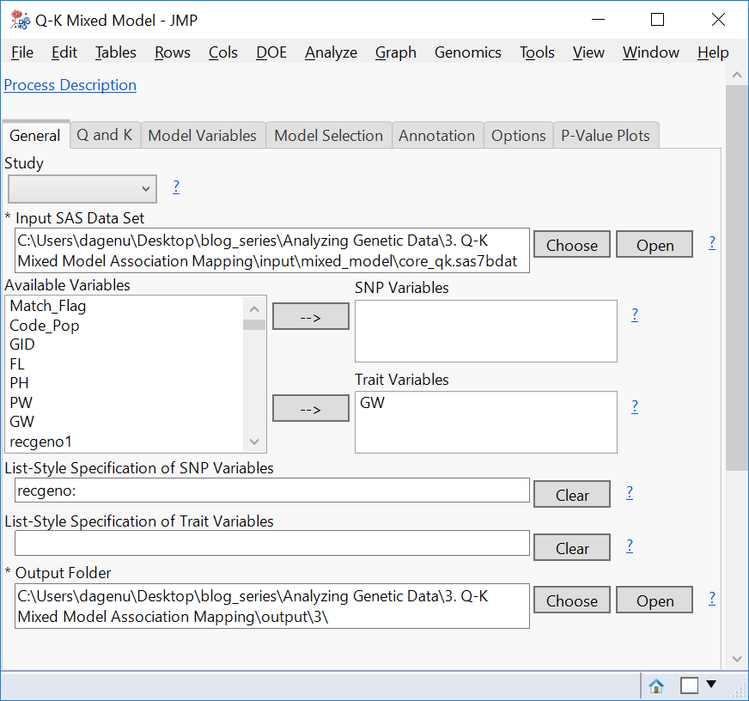
- Choose core_qk.sas7bdat as the Input SAS Data Set.
- Select GW as the Trait Variable.
- Enter recgeno: in the box under List-Style Specification of SNP Variables.
- Choose an Output Folder.
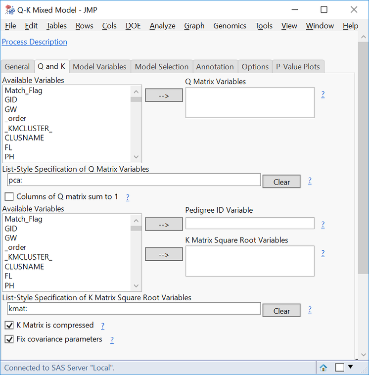
- On the Q and K tab, type pca: in the List-Style Specification of Q Matrix Variables box, and type IBD: in the List-Style Specification of K Matrix Square Root Variables
- If using the compressed K matrix, check the box K Matrix is compressed.
- On the Model Variables tab, select Continuous for Type of Trait. There are no additional effects in this data set.
- The Model Selection tab allows for the implementation of a multi-marker model, based on rotated markers and phenotypic variables. When selected, the user can choose from methods like ElassticNet, Stepwise, and LASSO. We will not fit a multi-marker model in this example.
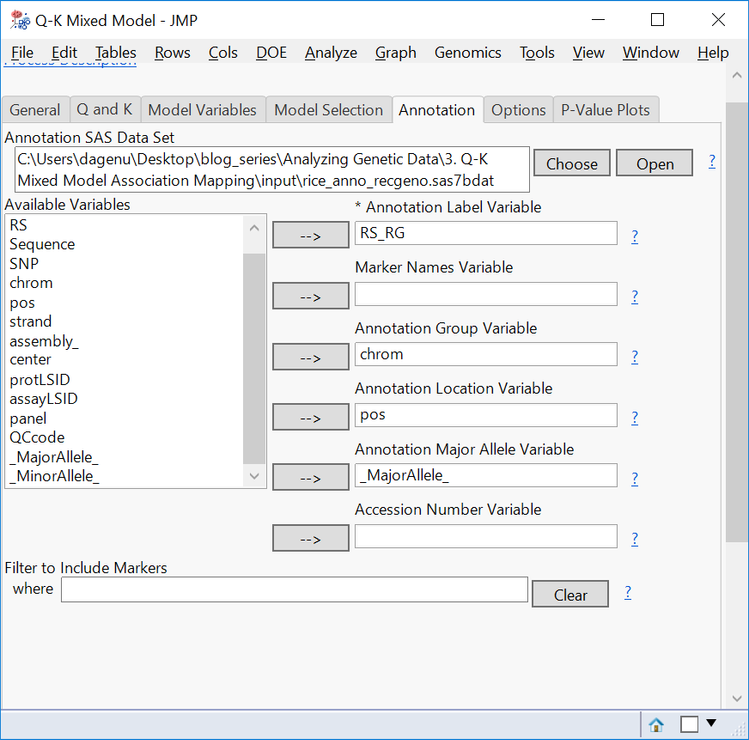
- On the Annotation tab, Choose rice_anno_recgeno.sas7bdat as the Annotation SAS Data Set.
- Fill out the Annotation tab with RS_RG as the Annotation Label Variable, chrom as the Annotation Group Variable, pos as the Annotation Location Variable, and _MajorAllele_ as the Annotation Major Allele Variable.
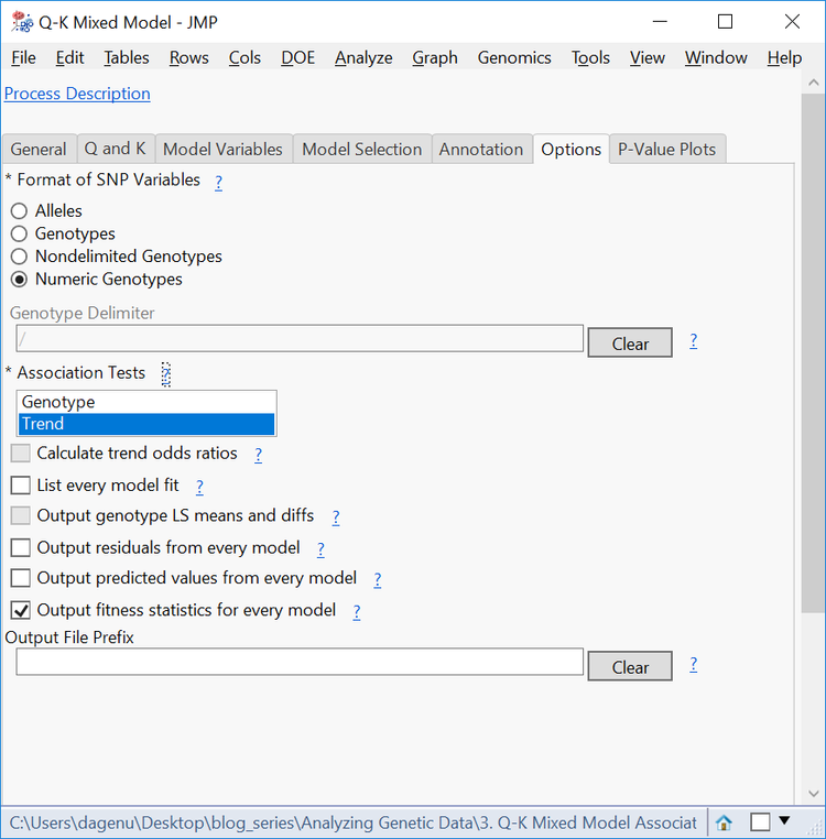
- On the Options tab, change the Format of SNP Variables to Numeric Genotypes.
- For a shorter computing time, deselect the Genotype Association Test. Optionally, the Genotype test performs chi-square tests based on genotypes, where the Trend test performs a Cochran-Armitage test.
- Click Run to start the analysis.
Results
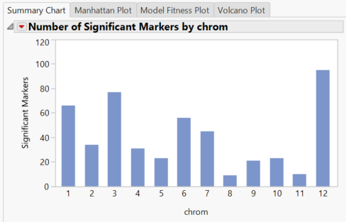
- When the results dashboard opens, the Summary Chart tab shows the number of significant markers on each chromosome for the Grain Yield (GW)
- The blue bars represent results from the Trend test. The trend test looks for a linear relationship in the trend scores when moving from homozygous minor to heterozygous to homozygous major.
- The blue bars represent results from the Trend test. The trend test looks for a linear relationship in the trend scores when moving from homozygous minor to heterozygous to homozygous major.
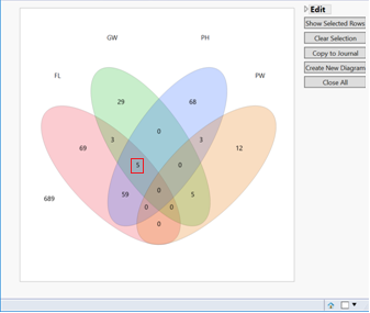
- When performing a model on multiple traits, significant markers that overlap across the traits can be viewed and data subsets can be created via a venn diagram output.
- There are five markers that are significant in common between GW, FL, and PH.
- There are five markers that are significant in common between GW, FL, and PH.
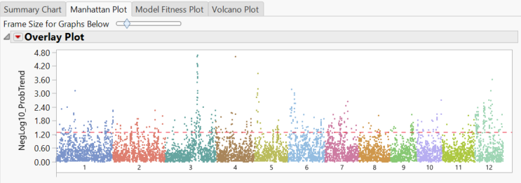
- The Manhattan Plot tab once again shows significant markers by chromosome as determined by the trend test.
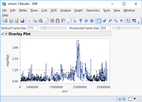
- Selecting any of the chromosomes from the Tabs menu on the left will bring up a plot of each marker on the chromosome plotted by position. Shown below is chrom 3 Results.
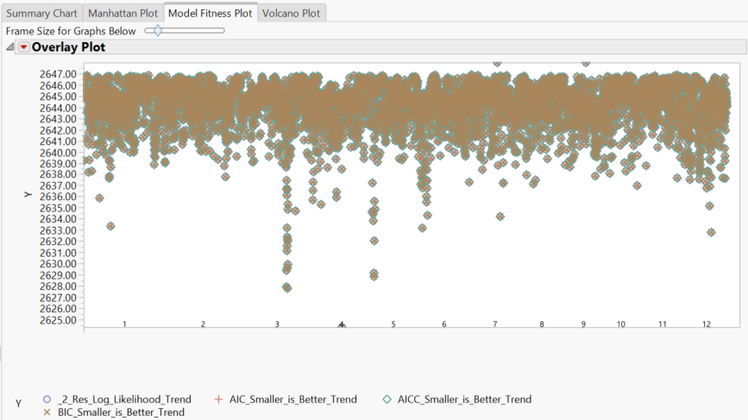
- The Model Fitness Plot tab shows fitness statistics for each marker. To separate the fitness plots by model, click the red triangle and select Overlay Plots > Overlay Ys. Tests are plotted by shape, with points lower on the plot representing higher accuracy.
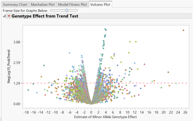
- The Volcano Plot tab gives a volcano plot for each marker, with minor allele genotype effect on the x-axis and the log transformed p-value on the y-axis. Points above the red line are considered significant.
- Clicking through the Local Data Filter options on the right will give volcano plots for each individual chromosome.
- Clicking through the Local Data Filter options on the right will give volcano plots for each individual chromosome.
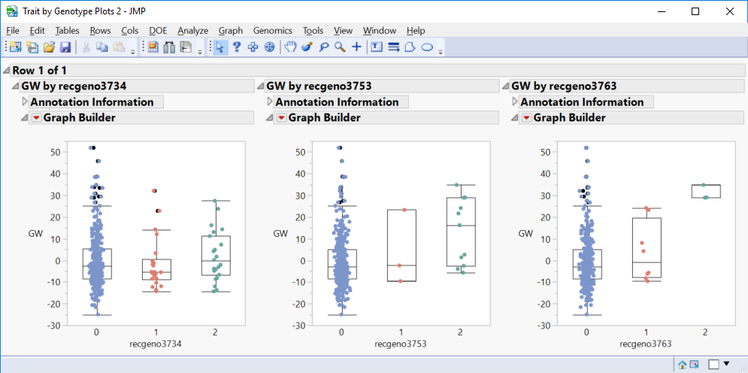
- In the Drill Downs menu, a subset can be created for selected markers, or a plot of Grain Yield values by genotype can be created by selecting Plot Trait By Genotype.
- This is a great way to quickly see the effect different genotypes have on a trait for a given marker.
- Shown below are trait by genotype plots, ordered by significance, from three markers on chromosome 5.
*The interactive results from this analysis are available on JMP Public.
Summary
This guide outlined the the Q-K Mixed Model process for association mapping while accounting for linkage disequilibrium caused by population structure and familial relatedness. QK analysis can be run in two different ways in JMP Genomics. A simpler option is the Genetics Q-K Analysis Workflow, which performs all the steps for the Q-K analysis and merges the data automatically. It is, however, less flexible than the process outlined in this post. The workflow only allows a Q matrix computed from PCA, and a K matrix from IBD calculations from the Relationship Matrix process. For detailed information on this process, see next week’s blog post: Part 3d: Q-K Mixed Model Genetic Association Workflow.
- © 2026 JMP Statistical Discovery LLC. All Rights Reserved.
- Terms of Use
- Privacy Statement
- Contact Us

You must be a registered user to add a comment. If you've already registered, sign in. Otherwise, register and sign in.