Vector Plots in JMP

[#1]

Vector plots show arrows on a two-dimensional plot and allow one to see four dimensions of data: x position, y position, arrow angle, and arrow length. Equivalently, the four dimensions can be x start position, y start position, x end position, and y end position. The latter form is most convenient for JMP. Though JMP doesn't have a menu command to create vector plots, arrows can be added to almost any plot without much trouble.

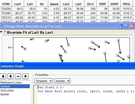
While lots of four-variable data sets can be adapted for vector display, I'll demonstrate with one of the most natural applications: wind data. This data set records wind speed and direction for various weather stations in the Chicago area. I used formulas to convert the speed and direction into end positions for the arrows and then added the following graphics script to a bivariate scatterplot using Customize from the graph's right-click menu.

Bivariate(
	Y( :Lat1 ),
	X( :Lon1 ),
	Show Points( 0 ),
	SendToReport(
		Dispatch( {}, "1", ScaleBox, {Min( -90.9505699180481 )} ),
		Dispatch( {}, "2", ScaleBox, {Min( 38.9936726055607 ), Max( 44.9620694317012 ), Minor Ticks( 0 )} ),
		Dispatch(
			{},
			"Bivar Plot",
			FrameBox,
			{Frame Size( 501, 429 ), Add Graphics Script(
				1,
				Description( "Script" ),
				Pen Size( 2 );
				For Each Row( Arrow( {lon1, lat1}, {lon2, lat2} ) );
			), Grid Line Order( 3 ), Reference Line Order( 2 )}
		)
	)
)

Here's a screen capture showing a little bit of the data table, graph, and customize dialog:Windcapture

The next steps were to delete the rows with no wind and to turn off the points in the graph.

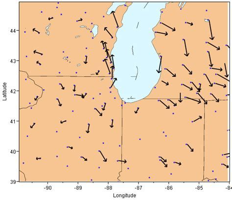
To provide context, I added the map of weather stations provided by the weather service. Placing a image in a graph is a bit tricky (and could be the subject of another post). There are two options: Draw the picture in another custom graphics script, or drag and drop an existing image into the graph. I chose the latter since I had an image file. First, I sized the graph to be the same size as the image, and then I dragged the image file into the center of the graph. After a few tries, the alignment was pretty good. (BTW, we're working on making this better in JMP 9.)Wind May31

The plot shows relative wind readings taken at 6 p.m. on May 31, 2009. With the help of the background image, we can see how wind patterns vary in relation to Lake Michigan.

The data file, with scripts, is available in the File Exchange, Chicago Wind Data and Plot 

Source of data and image: the National Severe Storms Laboratory Historical Weather Data Archives, Norman, Oklahoma.

[WP_Comment]

DaveG wrote:

hi,

note for readers - in JMP 9 you can take this script and add a background US map. Right click on the graph to customise, and select the US states map.

Great!

Dave

[WP_Comment]

Xan Gregg wrote:

Very nice -- that gives five dimensions of data, now.

The background image is discussed a little in the blog post. I dragged a PNG file in manually; unfortunately, it's not currently scriptable.

[WP_Comment]

Karen wrote:

Thanks Xan,

Very interesting and easy to follow. I didn't know you could add a script to a graph like that. I played with the examples and added the Pen Color line so that the arrow now takes its color from the table. Then i added a legend to the graph so it would color the rows by temperature and you end up with pretty colored arrows AND points.

How do you get the picture in the background in the screenshot on your blog?

Bivariate(
Y( :Lat1 ),
X( :Lon1 ),
SendToReport(
Dispatch(
{},
"Bivar Plot",
FrameBox,
{Frame Size( 501, 429 ),
Add Graphics Script(
2,
Description( "Script" ),
For Each Row(
Pen Color( Color Of( Row State() ) );
Pen Size( 2 );
Arrow( {:Lon1, :Lat1}, {:Lon2, :Lat2} );
)
), Row Legend(
TMPF,
Color( 1 ),
Color Theme( "Blue to Gray to Red" ),
Marker( 0 ),
Marker Theme( "" ),
Continuous Scale( 1 ),
Reverse Scale( 0 ),
Excluded Rows( 0 )
)}
)
)
)

[WP_Comment]

Xan Gregg wrote:

I uploaded the data file to the File Exchange under the name "ChicagoWind.jmp". It includes scripts that draw the plot with vectors.

[WP_Comment]

Karen wrote:

Hi Xan,

Can I get a copy of your vectorplot table with script? I would like to understand this capability better.

Thanks,

Karen

[WP_Comment]

Nishant Thakur wrote:

Hi, I am Nishant.I am trying this script but only Lat1 and Lon1 are getting plotted on graph. How should I plot Lat2 and Lon2 on same graph. Would you please guide me?

[XanGregg]

Xan Gregg wrote:

Did you add the custom script? That's what pulls in Lat2 and Lon2. You might try the script from Karen's comment above for a complete solution, and then work backwards to see how it differs from yours.

[WP_Comment]

Daryl Purcell wrote:

Is it possible to draw/append a line from the tip of one vector to another. would be very useful in residual analysis applications where user is interested in shape. Let me know. Thanks!

[XanGregg]

Xan Gregg wrote:

Of course you can do anything by modifying the script :). For instance, to operate on single x and y column, replace the Arrow command with something like If(row() > 1, Arrow({x[row()-1], y[row()-1]}, {x, y})).

Even without modifying the script, you can get the effect by chaining the x/y values in the table. That is, x1,y1 of row n would be the same as x2,y2 from row n-1.

[RyMcQeN]

Hello Xan,

I was wondering if you can suggest an efficient way to apply the arrows to multiple bivariate fit graphs (grouped by some other column).  For example, if I had multiple days worth of 'ChicagoWind' data and wanted to plot several bivariate charts by each date and apply the arrows by date.  Is there an easier way to do this rather than building a loop for each date?

Thank you,

Ry

[JanneI]

Hi Xan,

Same question than earlier from RyMcQeN; how one need to modify the script to get grouping by some other column? My scenario is from silicon industry; I would like to use vector graphs to so lithographic overlay error of stepper exposure tool over the silicon wafer (one vector per shot corner). My data contains multiple wafers and these could be used for grouping.

In graph builder, I would use Wrap for this. However, on GraphBuilder, I haven't find way to create vectors (I am running JMP15).

[Jeff_Perkinson]

@JanneI, the trick here is to apply your customization graphics script before you drag your column to wrap.

 

[mvanderaa1]

How would I go about only plotting for vectors for rows that are not excluded. Currently the scatter plot will not show the excluded rows, but their arrows are still plotted.

Edit: Ok it seems quite simple:

For Each Row(
    If( !Excluded(),
        Arrow( {:x, :y}, {:x + :dx, :y + :dy} )
    )
)

[pcncku2024]

Hi. Could someone share the link where I can download the JMP data file ("ChicagoWind.jmp"). I cannot find it. Thanks a lot.

[hogi]

 Chicago Wind Data and Plot 

I just noticed that Vector plots are "in the queue" to be implemented in a future version of JMP - nice
Add vector fields to Graph Builder