- New to JMP? Let the Data Analysis Director guide you through selecting an analysis task, an analysis goal, and a data type. Available now in the JMP Marketplace!
- See how to install JMP Marketplace extensions to customize and enhance JMP.
JMP Blog
A blog for anyone curious about data visualization, design of experiments, statistics, predictive modeling, and more- JMP User Community
- :
- Blogs
- :
- JMP Blog
- :
- The QbD Column: Is QbD applicable for developing analytic methods?
- Subscribe to RSS Feed
- Mark as New
- Mark as Read
- Bookmark
- Subscribe
- Printer Friendly Page
- Report Inappropriate Content
Editor's note: This post is by @ronkenett and @david_s of the KPA Group. It is part of a series of blog posts called The QbD Column. For more information on the authors, click the authors' community names above.


Development of measurement or analytic methods parallels the development of drug products. Understanding of the process monitoring and control requirements drives the performance criteria for analytical methods, including the process critical quality attributes (CQAs) and specification limits. Uncovering the characteristics of a drug substance that require control to ensure safety or efficacy determines the identification of CQAs. The typical requirements of analytic methods include:
- Precision: This requirement makes sure that method variability is only a small proportion of the specifications range (upper specification limit – lower specification limit). This is also called Gage Reproducibility and Repeatability (GR&R).
- Selectivity: This determines which impurities to monitor at each production step and specifies design methods that adequately discriminate the relative proportions of each impurity.
- Sensitivity: To achieve effective process control, this requires methods that accurately reflect changes in CQA's that are important relative to the specification limits.
These criteria establish the reliability of methods for use in routine operations. This has implications for analysis time, acceptable solvents and available equipment. To develop an analytic method with QbD principles, the method’s performance criteria must be understood, as well as the desired operational intent of the eventual end-user. Limited understanding of a method can lead to poor technology transfer from the laboratory into use in commercial manufacturing facilities or from an existing facility to a new one. Failed transfers often require significant additional resources to remedy the causes of the failure, usually at a time when there is considerable pressure to move ahead with the launch of a new product. Applying Quality by Design (QbD) to analytic methods aims to prevent such problems. QbD implementation in the development of analytic methods is typically a four-stage process, addressing both design and control of the methods[1]. The stages are:
- Method Design Intent: Identify and specify the analytical method performance.
- Method Design Selection: Select the method work conditions to achieve the design intent.
- Method Control Definition: Establish and define appropriate controls for the components with the largest contributions to performance variability.
- Method Control Validation: Demonstrate acceptable method performance with robust and effective controls.
Testing robustness of analytical methods involves evaluating the influence of small changes in the operating conditions[2]. Ruggedness testing identifies the degree of reproducibility of test results obtained by the analysis of the same sample under various normal test conditions such as different laboratories, analysts, and instruments. In the following case study, we focus on the use of experiments to assess and improve robustness.
A case study in HPLC development
The case study presented here is from the development of a High Performance Liquid Chromatography (HPLC) method[3]. It is a typical example of testing the robustness of analytical methods. The specific system consists of an Agilent 1050, with a variable-wavelength UV detector and a model 3396-A integrator. The goal of the robustness study is to find out whether deviations from the nominal operating conditions affect the results. Table 1 lists the factors and their levels used in this case study. The experimental array is a 27-4 Fractional Factorial experiment with three center points (see Table 2). The levels "-1" and "1" correspond to the lower and upper levels listed in Table 1, and "0" corresponds to the nominal level. The lower and upper levels are chosen to reflect variation that might naturally occur about the nominal setting during regular operation. For examples of QbD applications of Fractional Factorial experiments to formulation and drug product development, see the second and third blog posts in this series.
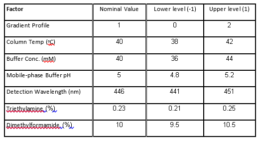
Table 1. Factors and levels in the HPLC experiment.
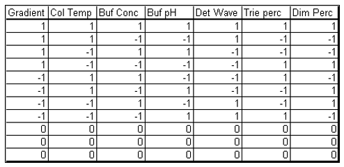
Table 2. Experimental array of the HPLC experiment.
The experimental array consists of 11 experimental runs that combine the design factors levels in a balanced set of combinations and three center points.
What we can learn from the HPLC experiments
In analyzing the HPLC experiment, we have the following goals:
- Find expected method measurement prediction variance for recommended setups of the method (the measurement uncertainty).
- Identify the best settings of the experimental factors to achieve acceptable performance.
- Determine the factors that impact the performance of the method on one or more responses.
- Assess the impact of variability in the experimental factors on the measured responses.
- Make robust the HPLC process by exploiting nonlinearity in the factor effects to achieve performance that is not sensitive to changes about nominal levels.
If we consider only the eight experimental runs of the 27-4 fractional factorial, without the center points, we get an average prediction variance of 0.417 and 100% optimality for fitting a first-order model. This is due to the balanced property of the design (see Figure 1 Left). The design in Table 2, with three center points, reduces prediction uncertainty near the center of the region and has a lower average prediction variance of 0.38. However, the center points don't contribute to estimating slopes, as seen in the lower efficiency for fitting the first-order model (see Figure 1 Right). 
Figure 1. Design diagnostics for this fractional factorial without (left) and with (right) three center points.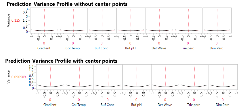
Figure 2. Prediction variance profile without (top) and with (bottom) center points.
The JMP Prediction Variance Profile in Figure 2 shows the ratio of the prediction variance to the error variance, also called the relative variance of prediction, at various factor level combinations. Relative variance is minimized at the center of the design. Adding three center points reduces prediction variance by 25%, from 0.12 to 0.09. This is an advantage derived by adding experimental runs at the center points. Another advantage that we will see later is that the center points permit us to assess nonlinear effects, or lack-of-fit for the linear regression model. A third advantage is that the center points give us a model-free estimate of the extent of natural variation in the system. At each factor level combination, the experiments produced five responses: 1) Area of chromatogram at peak (peakArea), 2) Height of chromatogram at peak (peakHeight), 3) Minimum retention time adjusted to standard (tRmin), 4) Unadjusted minimum retention time (unad tRmin) and 5) Chromatogram resolution (Res). Our first concern in analyzing the data is to identify proper models linking factors and responses.
What do we learn from analyzing the data from the fractional factorial experiment?
Linear regression models are the simplest models to consider. They represent changes in responses between two levels of factors, in our case this corresponds to levels labeled “-1” and “+1”. Since we also have three center points, at levels labeled “0”, we can also assess nonlinear effects. We do so, as in our second blog post, by adding a synthetic indicator variable designed to assess lack-of-fit (LOF) that is equal to “1” at the center points and “0” elsewhere. The JMP Effect Summary report, for all five responses with linear effects on all seven factors, and the LOF indicator, is presented in Figure 3. 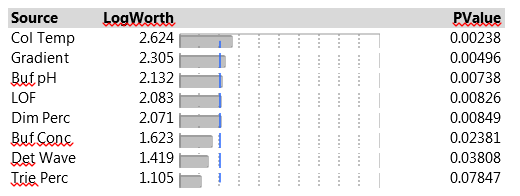
Figure 3. Effect Summary report of seven factors and LOF indicator on five responses.
The Effect Summary table lists the model effects across the full set of five responses, sorted by ascending p-values. The LogWorth for each effect is defined as -log10(p-value), which adjusts p-values to provide an appropriate scale for graphics. A LogWorth that exceeds 2 is significant at the 0.01 level because -log10(0.01)=2. The report includes a bar graph of the LogWorth with dashed vertical lines at integer values and a blue reference line at 2. The displayed p-values correspond to the significance test displayed in the Effect Tests table of the model report. The report in Figure 3 shows that, overall, four factors and LOF are significant at the 0.01 level (Col Temp, Gradient, Buf PH and Dim Perc) and Buf Conc, Det Wave and Trie Perc are non-significant. From the experimental plan in Table 2, one can estimate the main effects of the seven factors and the LOF indicator on the five responses with a linear model. Figure 4 presents parameter estimates for peakHeight with an adjusted R2 of 93%, a very good fit. The peakHeight response is most sensitive to variations in Col Temp, Det Wave and Gradient.
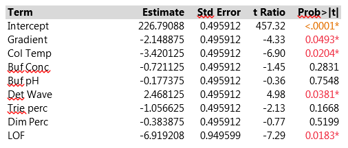
Figure 4. Parameter estimates of peakHeight of seven factors and LOF indicator with linear model. For improved readability, peakHeights have been divided by 1000.
We observe a statistically significant difference between the predicted value at the center point of the experimental design and the three measurements actually performed there (via the LOF variable). Figure 5 displays a profiler plot showing the linear effects of each factor on all five responses. The plot is very helpful in highlighting which conditions might affect the HPLC method. We see that Col Temp and Gradient, the two most important factors, affect several different responses. Buf pH, Buf Conc and Dim Perc have especially strong effects on the retention responses, but have weak effects on the other CQA's. The factors give good fits to the retention responses and to peakHeight, but not to peakArea or Res, which is reflected in the wide confidence bands for those CQA's and in high p-values for the overall model F-tests in the Analysis of Variance line of the model output.
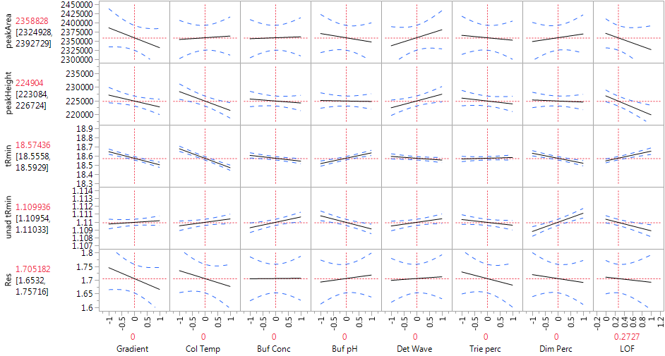
Figure 5. Profiler of HPLC experiments with linear model.
What should we do about the nonlinearity? Our analysis found a significant effect of the LOF indicator, which points to a nonlinear effect that is not accounted for in the profiler of Figure 5. The center points we added to the two-level fractional factorial design let us detect the nonlinearity, but they don’t provide enough information to determine what causes it – any one of the seven factors (and possibly several of them) could be responsible for the nonlinear effect on peak Height. In our next blog, we will discuss some design options to address the problem. For now, we show what we achieved with the current experiment. After much brainstorming, the HPLC team decided that it was very likely that the Gradient was the factor causing the nonlinearity. This important assumption, based only on process knowledge, is crucial to all our subsequent conclusions. We proceeded to fit a model to the original experimental data that includes a quadratic effect for Gradient. The team also decided to retain only the factors with the strongest main effects for each response; for peakHeight, the factors were Gradient, Column Temperature and Detection Wavelength. In Figure 6, we show parameter estimates from fitting this reduced model to the peakHeight responses. With this model, all terms are significant with an adjusted R2 of 89%. The root mean squared error, which estimates run-to-run variation at the same settings of the factors, is 1.754, slightly less than 1% the magnitude of peakHeight itself (after dividing peakHeight by 1000).
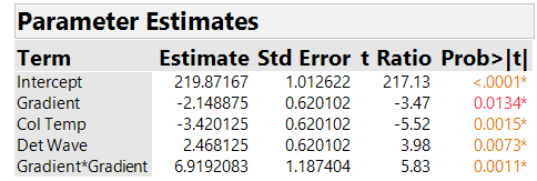
Figure 6. Parameter estimates of peakHeight with quadratic model. For improved readability, peakHeights have been divided by 1000.
We show a Profiler for the reduced quadratic model in Figure 7. 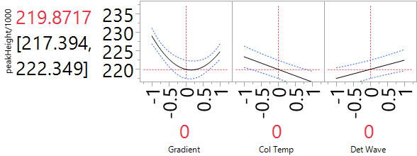
Figure 7. Profiler of HPLC experiment with reduced quadratic model for peakHeight. For improved readability, peakHeights have been divided by 1000.
Finding a robust solution
One of the main goals of the experiment was to assess the robustness of the system to variation in the input factors. We explore this question by introducing normal noise to the four factors in the reduced quadratic model. For each of the three factors, we assumed a standard deviation of 0.4 (in the coded units), which is the default option in JMP. This reflects a view that the experimental settings are about 2.5 SD from the nominal level, so reflect rather extreme deviations that might be encountered in practice. Figure 8 presents the effect of noise on peakHeight for a set-up at the center point which was initially identified as the nominal setting. We can compute the SD of the simulated outcomes by saving them to a table and using the “distribution” tab in JMP. The SD turns out to be 2.397 and is slightly larger than the run-to-run SD that we computed earlier of 1.754. The overall SD associated with the analytic system involves both of these components. To combine them, we need to first square them, then add them (because variances are additive, not SD) and then take a square root to return to the original measurement scale. The resulting combined SD is 2.970, so the anticipated variation in factor settings leads to an SD about 70% larger than the one from run-to-run variation alone. The overall SD is less than 1.5% of the typical values of peakHeight and that was considered acceptable for this process.
Is our nominal solution a good one for robustness?
Figure 8 is very helpful in answering this question. The important factor here is Gradient, through its non-linear relationship to peakHeight. The “valley” of that relationship is near the nominal choice of 0. Our simulation of factor variation generates values of Gradient that cover the range from -1 to 1. When those values are in the valley, they transmit very little variation to peakHeight. By contrast, when they are near the extremes, there is substantial variation in peakHeight. So the fact that the bottom of the valley is close to the nominal setting assures us that the transmitted variation will be about as small as possible. We can test this feature by shifting the nominal value of Gradient. When the nominal is -0.5, the simulator shows that the SD from factor variation increases to 4.282, almost 80% more than for the nominal setting at 0. The dependence of peakHeight on Col Temp and on Det Wave is linear. So regardless of how we choose the nominal settings of these factors, they will transmit the same degree of variation to the peakHeight output. The experiment lets us assess how they affect robustness, but does not provide any opportunity to exploit the results to improve robustness.
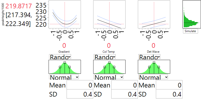
Figure 8. Prediction Profiler of peakHeight when the factors are at their nominal settings and the natural SD is 0.4. For improved readability, peakHeights have been divided by 1000.
Going back to the original questions
In reviewing the questions originally posed, we can now provide the following answers:
1. What is the expected method measurement prediction variance for recommended set ups of the method (the measurement uncertainty).
Answer: We looked at this question most closely for peakHeight, where we found that the SD is 2970, with roughly equal contributions from run-to-run variation and from variation in the measurement process factors.
2. What setup of the experimental factors will achieve acceptable performance?
Answer: With all factors at their nominal settings (coded value at 0), the SD of 2970 is less than 1.5% the size of the values measured, which is an acceptable level of variation in this application.
3. What are the factors that impact the performance of the method in one or more responses?
Answer: The three factors with highest impact on the method’s performance are gradient profile, column temperature and detection wave.
4. Can we make the setup of the experimental factors robust in order to achieve performance that is not sensitive to changes in factor levels?
Answer: We saw that we can improve robustness for peakHeight by setting the gradient to its coded level of 0 (the nominal level in the experiment). That setting helps us to take advantage of the non-linear effect of gradient and reduce transmitted variation.
5. Can we assess the impact of variability in the experimental factors on the analytical method?
Answer: As we noted earlier, the natural variability of the input factors is responsible for slightly more than half the variation in peakHeight.
Wrap-Up
In reviewing the questions originally posed, we first fit a linear regression model. After realizing that there is an unaccounted nonlinear effect we used a reduced quadratic model and found that it fits the data well. Inducing variability in the factors of the reduced quadratic (gradient profile, column temperature and detection wave), we could estimate of the variability due to the method and could assess the robustness of the recommended setup. The team’s assumption that gradient is responsible for the non-linearity is clearly important here. If other factors also have non-linear effects, there could be consequences for how to best improve the robustness of the method. We will explore this issue further in our next blog post.
Notes
[1] Borman, P., Nethercote, P., Chatfield, M., Thompson, D., Truman, K. (2007), Pharmaceutical Technology. http://pharmtech.findpharma.com/pharmtech/Peer-Reviewed+Research/The-Application-of-Quality-by-Desig...
[2] Kenett, R.S, and Kenett, D.A (2008), Quality by Design Applications in Biosimilar Technological Products, Accreditation and Quality Assurance, Springer Verlag, Vol. 13, No 12, pp. 681-690.
[3] Romero R., Gasquez, D., Sanshez, M., Rodriguez, L. and Bagur, M. (2002), A geometric approach to robustness testing in analytical HPLC, LCGC North America, 20, pp. 72-80, www.chromatographyonline.com.
You must be a registered user to add a comment. If you've already registered, sign in. Otherwise, register and sign in.
- © 2026 JMP Statistical Discovery LLC. All Rights Reserved.
- Terms of Use
- Privacy Statement
- Contact Us
