- Instantly extract effect sizes, F-ratios, and FDR-adjusted p-values from your models with the Calculate Effects Sizes extension, available now in the JMP Marketplace!
- New to JMP? Join us Sept. 23-24 for the Early User Edition of Discovery Summit, tailor-made for new users. Register now for free!
- Your voice matters! Tell us how you prefer to receive JMP updates, so we can tailor our communication to your needs. Take short survey.
JMP Blog
A blog for anyone curious about data visualization, design of experiments, statistics, predictive modeling, and more- JMP User Community
- :
- Blogs
- :
- JMP Blog
- :
- The QbD Column: Achieving robustness with stochastic emulators
- Subscribe to RSS Feed
- Mark as New
- Mark as Read
- Bookmark
- Subscribe
- Printer Friendly Page
- Report Inappropriate Content

Editor's note: This post is by @ronkenett, Anat Reiner-Benaim and @david_s of the KPA Group. It is part of a series of blog posts called The QbD Column. For more information on the authors, click the authors' community names above.


In an earlier installment of The QbD Column titled A QbD factorial experiment, we described a case study where the focus was on modeling the effect of three process factors on one response, viscosity. Here, we expand on that case study to show how to optimize process parameters of a product by considering eight responses and considering both their target values and the variability in achieving these targets. We apply a stochastic emulator approach, first proposed in Bates et al, 2006, to achieve robust on target performance. This provides additional insights to the setup of product and process factors, within a design space.
A case study with eight responses and three process factors
The case study refers to a formulation of a generic product designed to match the properties of an existing brand using in vitro tests. In vitro release is one of several standard methods used to characterize performance of a finished topical dosage form (for details see SUPAC, 1977).
The in vitro release testing apparatus has six cells where the tested generic product is compared to the brand product. A 90% confidence interval for the ratio of the median in vitro release rate in the generic and brand products is computed, and is expressed as a percentage. If the interval falls within the limits of 75% to 133.33%, the generic and brand products are considered equivalent.
The eight responses listed in the SUPAC standard that are considered in setting up the bioequivalence process design space are:
- Assay of active ingredient
- In vitro release rate lower confidence limit
- In vitro release rate upper confidence limit
- 90th percentile of particle size
- Assay of material A
- Assay of material B
- Viscosity
- pH values
Three process factors are considered:
- Temperature of reaction
- Blending time
- Cooling time
The experimental design consisted of a 23 factorial experiment with two center points. The experimental array and the eight responses are presented in Figure 1.
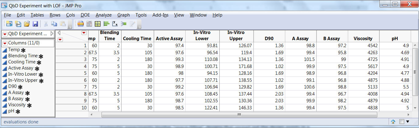
Figure 1: Experimental array and eight responses in QbD steroid lotion experiment
Fitting a model with main effects and interactions to the three process factors
Figure 2 shows the model we fitted to the data. It included main effects for each of the three factors and all the two-factor interactions. We used the same model for all the responses.
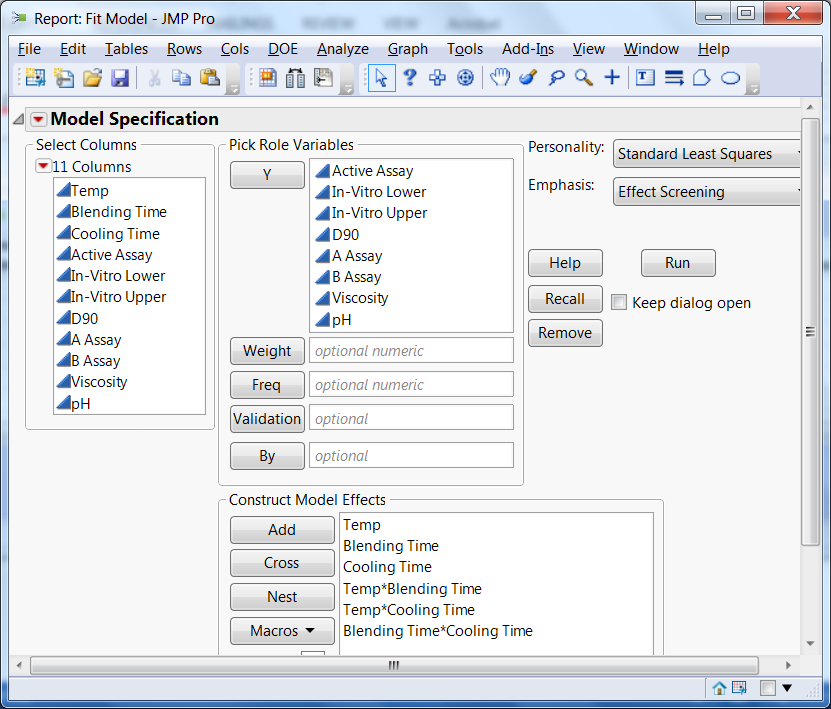
Figure 2: Model used to fit the QbD experimental data on all eight responses
Assessing operating conditions with the Profiler
The design was centered at the current “best guess” for operating conditions, with Temp=67.5, Blending Time=3.5 and Cooling Time=105. The fitted models at these values give an overall desirability index of 0.30 (for a description of desirability functions, see the second blog post in our QbD series titled A QbD factorial experiment). The resulting solution increases the Temperature to 75, reduces the Blending Time to 2 and sets the Cooling Time at 113.1, with a desirability of 0.54. Overall, our goal is to reduce defect rates.
If production capability allowed us to set the factor levels with high precision, the above solution would be a good one. However, there is always some uncertainty in production settings, with corresponding variation in process outputs. We now study the effect of this uncertainty, using computer simulations to reflect the variation in the design factors. We use the “simulator” option that is available with the Profiler in JMP.
The simulator opens input templates for each experimental factor and for each response, where we describe the nature of variation. For example, we set up the temperature to vary about its nominal value with a normal distribution and a standard deviation of 3 degrees. Describing variation in the outputs allows us to reflect the natural variation in output values about the expected value from the model. The standard deviations for the outputs could be the residual standard deviations from fitting the models. Clicking on the “simulate” key generates data for each output that is characteristic of typical results in regular production.
Figure 3 (below) shows simulated results based on our QbD experiment when all factor are set to their center values. The summary also shows that more than 80% of the simulated results do not meet process requirements and that these “out of spec” problems are all due to having an in vitro upper confidence limit that is too high.
The results in Figure 3 show that the center point is not a good operating condition and will have a high fraction of production out of spec. Moving the settings to maximize the desirability reduces the percent out of spec to 18%.
Using the simulator to find better operating conditions
We now take a further step and show how to use the simulator to find robust operating conditions that maintain high desirability and also reduce the percent out of spec. This can be done directly with the Profiler, moving the operating conditions with the slider bars and observing the results for desirability and percent defect. We present here a much more systematic approach based on a “computer experiment” to model the defect rate over the factor space.
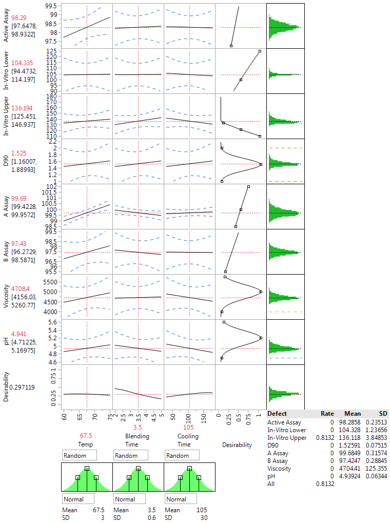
Figure 3: Assessing production at the center point from the QbD steroid lotion experiment with the JMP Profiler and the simulator option
Running experiments on computers
The simulator option in the JMP Profiler allows us to compare operating conditions via computer generated values that represent the natural production variation about target settings for the design factors. We continue our study, exploring how the factors will affect production by choosing a collection of points in the factor space at which to make these evaluations.
Such computer experiments, as opposed to physical experiments, typically use “space-filling” designs that spread out the design points in a more-or-less uniform fashion. Another characteristic of such experiments is that the data does not involve experimental error since, rerunning the analysis on the fitted model, at the same set of design points, will reproduce the same results.
In modeling data generated from computer experiments, different approaches are used, with Gaussian process models (also known as Kriging models) being the most popular. A key publication in this area is Sacks et al. (1989), which coined the term design and analysis of computer experiments (DACE).
Assessing the QbD study by a computer experiment
Our computer experiment for the formulation experiments used a 128-run space-filling design in the three experimental factors (the default design suggested by JMP). At each of these factor settings, the production variability is simulated, giving computer-generated responses as seen in Figure 3. Key indicators are used to summarize the responses at each setting. Then, we model the key indicators to see how they relate to the factor settings and to suggest optimal settings. Here, we focus our analysis on achieving high desirability and low defect rate.
Optimizing desirability of performance and defect rates
Maximizing the overall desirability, as shown earlier, leads to a new setup of the process factors (Temp=75, Blending Time=2, Cooling Time=113.1) with an overall desirability of 0.54 and an overall defect rate of 0.18. A 128 point space-filling experiment on the model, with no added errors on the responses, produced the data shown in Figure 4.
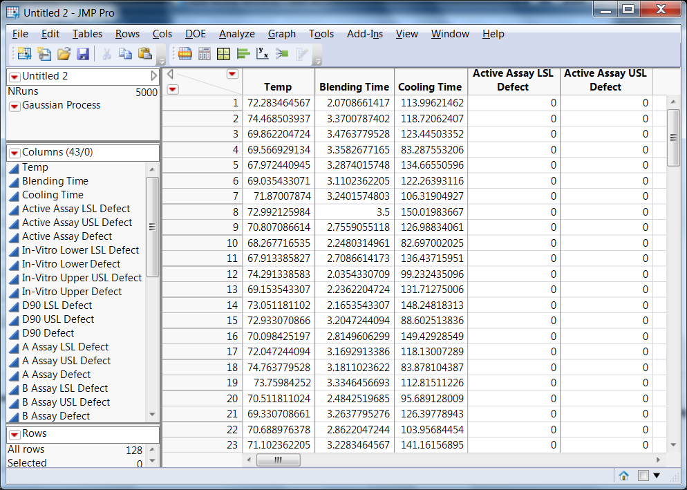
Figure 4: Results from space filling simulated experiments using model used to fit the QbD steroid lotion experimental data (the stochastic emulator data)
The Gaussian process model automatically generated by JMP is a natural tool for analyzing the data, and it opens in the data table of the computer experiment outcomes. The fitted model provides an emulator of the defect rate derived from adding production noise to the factor settings from the original model that was fit to the data. Since minimal is best in a defect rate, the optimization of this emulator model leads to a Profiler set at values minimizing defect rates. To apply these proposed values to the Profiler of the original model shown in Figure 3, one needs to link the profiles in the factor setting options. In Figure 5 we present the optimized Profiler on defect rate using the Gaussian model for fitting the stochastic emulator model derived from data generated from the original QbD model.

Figure 5: Optimized Prediction Profiler (minimizing defect rate) of stochastic emulator data.
The stochastic emulator
The optimization and robustness analysis above follows the “stochastic emulator” approach proposed by Bates el al. (2006). The approach is useful whenever there is a model that can describe input-output relationships and a characterization of sources of variability. The analysis can then be used to optimize a response by accounting for both its target values and variability. The stochastic emulator is used to model the variability in the data and, combined with optimization of a model fit to the physical experiments, allows us to ensure, as best as possible, both on-target performance and minimal variability. The key steps of the stochastic emulator approach are as follows:
- Begin with a model that relates the input factors to the system outputs. The model could be derived from the results of an initial laboratory experiment, as in our example here, or it could be derived on purely theoretical grounds from the basic science of the system.
- Characterize the uncertainty in the system. Describe how the input factors are expected to vary about their nominal process settings. The corresponding distributions are called noise distributions for the input factors. Describe the extent of output variation about the values computed from the model.
- Lay out an experimental design in the input factors that describes possible nominal settings. As noted earlier, space-filling designs are the popular choice here.
- Generate simulated data from the noise distributions at all the nominal settings in the space-filling design.
- Summarize the simulated data at each nominal setting by critical response variables (like desirability and defect rate in our study).
- Construct statistical models that relate critical response variables to the design factor settings using the Gaussian process model option in JMP.
- Optimize the choice of the factor settings for all critical outcomes. Here we want the process to have both on target performance and robustness (JMP allows us to do this by linking and optimizing Profilers).
Some concluding remarks
When we run the simulation on the noise in the design factors (Figure 3) at the set points achieved in Figure 5, (Temp=75, Blending Time=2, Cooling Time=150.6), we achieve an overall desirability of 0.53 and a defect rate of 0.09. This setup is slightly worse than the setup optimized only on performance relative to target but significantly better in terms of robustness.
Figure 5 suggests the possibility of achieving further reduction in the defect rate by moving the temperature and cooling time to higher levels and the blending time to lower levels. We set the factor ranges in our computer experiment to match the ones used in the experiment (but limited to values between the original operating proposal and the extreme experimental level in the direction we found best for robustness). We did not want to make predictions outside the experimental region, where our empirical models might no longer be accurate. In the context of QbD drug applications, extrapolation outside the experimental region is not acceptable.
In cases like this, it is often useful to carry out further experiments to explore promising regions. Extending the factor ranges in the directions noted above would let us model the responses there and assess the effects of further changes on robustness. For this application, the project team achieved a solid improvement and chose not to continue the experiment. In future blog posts, we will illustrate the benefits of including more than one phase in the QbD experimental program.
Stochastic emulators are a primary Quality by Design tool, which naturally incorporates simulation experiments in the design of drug products, analytical methods and scale-up processes. (For more on computer experiments and stochastic emulators see, Santner et al., 2004; Steinberg and Kenett, 2006; Levy and Steinberg, 2010; Kenett and Zacks, 2014.) For more examples of such experiments in the context of generic product design, see Arnon (2012, 2014).
We showed in this blog post, how a combination of physical full factorial experiments with a stochastic emulator leads to robust set up within a design space.
Coming attraction
The next blog post will be dedicated to mixture experiments and compositional data where the main interest is on the relative values of a set of components (which typically add to 100%) so that the factors cannot be changed independently.
References
- Arnon, M, (2012), Essential aspects in the ACE and ANDA IR QbD case studies,
- The 4th Jerusalem Conference on Quality by Design (QbD) and Pharma Sciences, Jerusalem, Israel, http://ce.pharmacy.wisc.edu/courseinfo/archive/2012Israel/
- Arnon, M. (2014). QbD In Extended Topicals Perrigo Israel Pharmaceuticals, The 4th Jerusalem Conference on Quality by Design (QbD) and Pharma Sciences, Jerusalem, Israel. https://medicine.ekmd.huji.ac.il/schools/pharmacy/En/home/news/Pages/QbD2014.aspx
- Bates, R., Kenett R.S., Steinberg D.M. and Wynn, H. (2006). Achieving Robust Design from Computer Simulations. Quality Technology and Quantitative Management, Vol. 3, No. 2, pp. 161-177.
- Kenett, R.S. and Steinberg, D.M. (2006). New Frontiers in Design of Experiments, Quality Progress, pp. 61-65, August.
- Kenett, R.S. and Zacks, S. (2014). Modern Industrial Statistics: with applications in R, MINITAB and JMP, John Wiley and Sons.
- Levy, S. and Steinberg, D.M. (2010). Computer experiments: a review. ASTA – Advances in Statistical Analysis, 94, 311-324.
- Sacks, J., Welch, W.J., Mitchell, T.J. and Wynn, H.P. (1989). Design and analysis of computer experiments. Statistical Science, 4, 409-435.
- Santner, T.J., Williams, B.J. and Notz, W.L. (2004). The Design and Analysis of Computer Experiments, Springer, New York, NY.
- SUPAC (1997) Food and Drug Administration, Center for Drug Evaluation and Research (CDER) Scale-Up and Postapproval Changes: Chemistry, Manufacturing, and Controls; In Vitro Release Testing and In Vivo Bioequivalence Documentation, Rockville, MD, USA.
You must be a registered user to add a comment. If you've already registered, sign in. Otherwise, register and sign in.
- © 2026 JMP Statistical Discovery LLC. All Rights Reserved.
- Terms of Use
- Privacy Statement
- Contact Us