- New to JMP? Let the Data Analysis Director guide you through selecting an analysis task, an analysis goal, and a data type. Available now in the JMP Marketplace!
- See how to install JMP Marketplace extensions to customize and enhance JMP.
JMP Blog
A blog for anyone curious about data visualization, design of experiments, statistics, predictive modeling, and more- JMP User Community
- :
- Blogs
- :
- JMP Blog
- :
- Piecewise Nonlinear Solutions Part 4: Using JMP's Nonlinear platform to solve fo...
- Subscribe to RSS Feed
- Mark as New
- Mark as Read
- Bookmark
- Subscribe
- Printer Friendly Page
- Report Inappropriate Content
This is the fourth of a series of posts on how to fit piecewise continuous functions to data sets. I like to begin each post with links to all of the other previous posts in the series:
- Part 1: Description of the problem, introduction of example data
- Part 2: Choosing functions that we want to fit, and setting boundary conditions between piecewise se...
- Part 3: Using JMP's Formula Editor to solve for unknown parameters
- Part 4: Choosing convergence criteria and algorithms, and running the Nonlinear platform to get parameters to converge
On to part 4...
Introduction
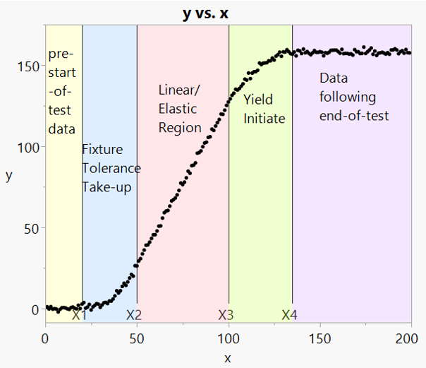
In previous posts in this series, we have been working on the data set shown in the following graph:
So far we have discussed segmenting the data regions and defining curves associated with each region, including:
- Eliminating some coefficients of the segmented equations by virtue of continuity at the endpoints.
- Using JMP's Formula Editor with unknown parameters and multiple equations all in one formula, in preparation for solving for the unknowns.
Now we are ready to use JMP's Nonlinear platform to find the unknown parameters and give a best-fit model. Now we discuss:
- How to solve the piecewise equations using JMP's Nonlinear platform
- Getting models to converge through:
- Optional convergence algorithms
- Setting parameter limits
- Convergence goals
Let's take a closer look.
JMP's Nonlinear Platform
The Nonlinear platform uses one of several user-selectable iterative estimation process to solve for the unknown parameters described in the Formula Editor. To solve the piecewise equations as described in previous blog posts, we first go to Analyze-->Specialized Modeling-->Nonlinear. The following user interface opens:
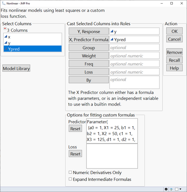
In Figure 2, we have already filled out the inputs.
- "Y, Response" is the original (measured) data.
- "X, Predictor Formula" is the formula column defined in the previous blog post.
- Note that the x values at which y values were measured are not input directly into the GUI, but are included via references in the formula column.
- Note that the parameters from the formula column are shown (along with their starting values) in the Options/Predictor section. JMP populates this automatically for us.
After clicking OK, the following window appears:
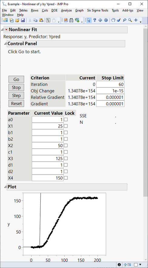
Here we see a summary of the model so far, with starting values shown for each unknown parameter. We also see the convergence criterion (discussed later). We see the original data (black dots) and the current fit (thin black line, resulting from using parameter starting values).
We also have four buttons:
- Go: Starts the iterative solver process.
- Stop: Stops the process (if the solver is not converging).
- Step: Manually takse one iteration step at a time, to watch how the convergence criterion and fit plot are changing.
- Reset: Resets the parameters to their starting values.
Clicking the "Step" button a few times, we can see the convergence algorithm at work:
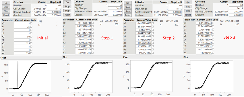
In the subplots of Figure 4, note that the thin black line is definitely converging toward the measured data as we increment the steps. In addition, the parameters are changing, and the convergence criteria are shrinking as well.
Clicking the Go button automatically brings us to the final converged values, as shown below:
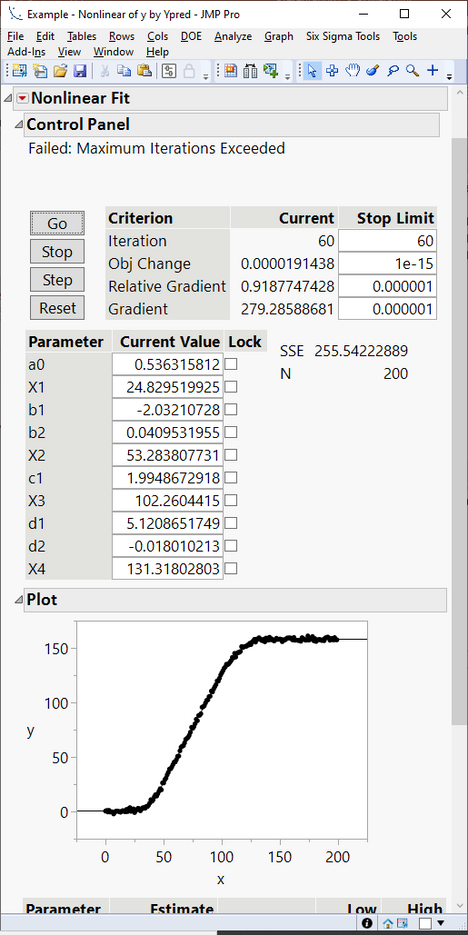
In Figure 5, at the top of the output we have a warning message that reads "Failed: Maximum Iterations Exceeded." We will talk about that later in this post. But looking at the plot, it is clear that we have already achieved good convergence of the model with the observed data.
Some observations about the parameters:
- Recall from Figure 1 that X1, X2, X3, and X4 were the cutpoints of the piecewise functions. These have shifted appropriately from their estimated starting values to give good endpoints for each of the piecewise functions.
- The remaining parameters all have importance for the individual curve pieces. For example, a0 represents the average Y level before test data begins to accumulate at X1=24.8.
What happens if we don't have convergence?
Options for When the Solution Does Not Converge
As noted above, this particular solution did not (technically) converge. This means that the default convergence algorithm did not meet its convergence criteria, as defined in the Nonlinear Fit control panel. In fact, without convergence, JMP doesn't let us do much with the results (like save the new parameters).
So what can we do? There are several options:
Change the Convergence Criteria
In the Criterion section of Figure 5, we can see what the current convergence criteria are, and how close we are to meeting them. For example, JMP went through 60 iteration steps in the previous example and did not achieve convergence. So we might want to increase the "stop limit" to try more steps (at the expense of taking longer to converge.)
Or we may wish to change either Obj Change, Relative Gradient, or Gradient. Convergence is achieved if any one of the three criteria fall below the "Stop Limit."
Change the Iterative Estimation Algorithm
The red triangle next to "Nonlinear Fit" (see Figure 3) gives several options, including "Iteration Options." Here we have three different iteration algorithms to choose from:
- Newton (the default)
-
Quasi-Newton BFGS
-
Quasi-Newton SR1
Some of these options also allow computation of "Numeric Derivatives Only." Per JMP Help, there is no consensus on which of these algorithms is the best to use, as it depends on the particular data and equation being fit.
You can combine the algorithms. For example, in our test case the Newton method did not converge. But you can retain the values that the Newton method arrived at, and simply change the iteration algorithm, and then click the Go button to proceed with convergence from the endpoint achieved by the Newton algorithm. Why does this work? Because we are starting with better estimates of the parameters.
Which brings me to my next option to improve convergence...
Setting Parameter Limits
Sometimes when an iterative algorithm adjusts a parameter, it can "take off" in the wrong direction or get stuck in a local minimum, etc. When this happens, it may be beneficial to limit the ranges that parameters can take.
In our example problem, perhaps we know that the X1 cutoff point should have a value of about 20. We might want to tell JMP that X1 must not fall outside the range 15-25. This will help prevent the iterative algorithm from "getting lost" as it does its work.
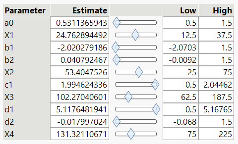
Parameter Bounds can be found under the same Nonlinear Fit red triangle. Once activated, a table appears at the bottom of the report, allowing you to input estimates and ranges for each variable. Also of note is that you can use the sliders in this table as a sort of Profiler, to examine the effects of changing each parameter on the overall fit shown in the plot.
Figure 6 shows an example of the Parameter Bounds table:
Once We Have Achieved Convergence
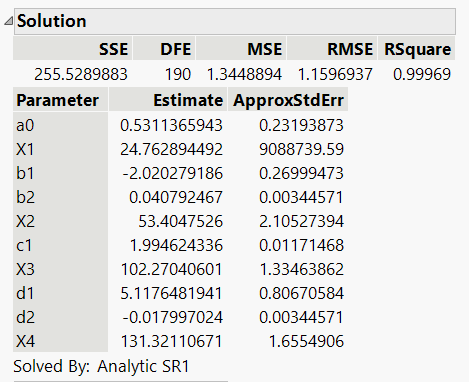
If you have a proper equation formed in the Formula Editor, and you have achieved convergence via the options described above, then JMP's Nonlinear platform should have provided the best estimates of all unknown parameters. You will see a note to the effect "Converged in Gradient" at the top of the report, and at the bottom of the report you will see a section for "Solution", showing the final estimates of all unknown parameters:
Also, just above the plot of measured data and best fit function, there should now be a button to "Save Estimates." Clicking this button will replace the current parameter values in the formula with the new best-fit values.
You must be a registered user to add a comment. If you've already registered, sign in. Otherwise, register and sign in.
- © 2026 JMP Statistical Discovery LLC. All Rights Reserved.
- Terms of Use
- Privacy Statement
- Contact Us
