This is the second of a series of posts on how to fit piecewise continuous functions to data sets. I'll begin each post with links to all of the other posts in the series. They are:
This post, by necessity, is a little "math-y."
Introduction
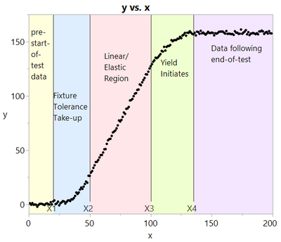
In Part 1 of this blog series, I introduced an example problem to demonstrate something called "fitting piecewise functions" to a dataset. These data were broken into regions where we would like to fit (as yet TBD) functions. Even the X locations that define the boundaries of the regions are as yet unknown. Figure 1 shows the data and the suggested regions.
 Figure 1
Choosing Functions
For each region, we wish to fit different functions that serve to model the data. In JMP's Nonlinear platform, you can use any expression that you like (e.g. exponentials, logs, trigonometrics, etc.) In general, selection of the functions will be entirely up to the wisdom, insight, and subject matter expertise of the modeler. The following discussion uses simple polynomials, which offer the benefit of simplifying math when it comes to establishing boundary conditions. These have worked well for me over the years.
By simple polynomial, I mean an equation of the form:
 Equation 1
where:
y = the measured response
n = the segment of interest
Am = the "mth" unknown coefficient for the nth segment
x = the independent predictor
The polynomial can be truncated to any desired length, depending on the complexity of the function to be fit.
Let's look at each segment of Figure 1 individually.
Segment 1: Pre-start-of-test data
As described earlier, this region might consist of data that are collected before the test actually starts. In this case, it might ideally have a y value of zero, though there could be some instrumentation offset. We expect this to be a constant value, so we would set the polynomial for the first segment as:
 Equation 2
Segment 2: Fixture Tolerance Take-up
Recall that the example data set might represent data from a tensile test machine, where a specimen is placed in the tester using a mounting figure. The second segment/region shown in Figure 1 (between X1 and X2) might indicate a region where fixture tolerances are being taken up. We might be interested primarily in how much take-up there is (X2-X1), or in how much force is required to take out all of the tolerance.
Since there is curvature in this region, I chose to use a quadratic function for the fit. I also chose to change the parameters to b's instead of a's, just to help distinguish the coefficients in this segment from those in Segment 1:
 Equation 3
Segment 3: Linear/Elastic Region
Segment 3 might be the most important region for the test, since our goal is to understand the elastic region of the curve. Here the relationship between x and y is linear, perhaps representing the elastic region for our example test specimen in the tensile fixture. We would be most interested in the slope of this region, so I chose a simple slope-intercept form for this equation:
 Equation 4
Segment 4: Yield Initiates
Segment 4 might cover the area in our example test data where our tensile specimen begins to yield. Visual inspection of the data shows that there is curvature again (similar to Segment 2), so again I chose a quadratic fit:
 Equation 5
Segment 5: Data Following End of Test
Segment 5 might occur after the actual tensile test has finished. The test specimen is still under tension. The amount of stretch (y) is unchanging, so the equation would be similar to Segment 1:
 Equation 6
Setting Boundary Conditions
We now have five equations with unknown coefficients (a0, b0, b1, b2, c0, c1, d0, d1, d2, and e0) along with the four breakpoints X1, X2, X3, and X4. Each of these needs to be determined. But there is more information that needs to be provided. Specifically, each of the curves needs to "connect" at the transition boundaries.
Segment 1 to Segment 2 transition
For the Segment 1/2 transition, we want y1=y2 at x=X1. This means:
 Equation 7
Solving for b0, we get:
 Equation 8
This "connects" the function of Segment 1 with the function of Segment 2 at x=X1. This gives us a way to eliminate b0 from any upcoming equations.
Remaining segment boundaries
Without spelling out all of the algebra, we can do the same thing with each of the other boundaries (e.g. y2(X2) = y3(X2), etc.). Solving for c0, d0, and e0, we arrive at:
 Equation 9
 Equation 10
 Equation 11
After making multiple substitutions into the segment equations, we arrive at:
 Equation 12
 Equation 13
 Equation 14
 Equation 15
 Equation 16
So now we have whittled down the unknowns to a0, b1, b2, c1, d1, d2, X1, X2, X3, and X4. How do we get JMP to solve for these unknowns? Join me for the next blog post!
You must be a registered user to add a comment. If you've already registered, sign in. Otherwise, register and sign in.