Piecewise Nonlinear Solutions Part 3: Using JMP's Formula Editor to solve for unknown parameters

JerryFish · Oct 28, 2021 12:31 PM

This is the third of a series of posts on how to fit piecewise continuous functions to data sets. I'll begin each post with links to all of the other posts in the series. They are:

Onto part 3...

Introduction

If you have followed along with my previous posts in this series, you know that we have now developed equations containing 10 unknown parameters that need to be determined in order to best fit the pieces of the example problem. How do we do this in JMP?

First, we need to use JMP's Formula Editor to input our equations and unknown parameters. I will assume that the reader is generally familiar with the Formula Editor. (If not, here is a short video on Creating Formulas and a longer video with much more detail on the Formula Editor.)

Setting up Parameters in JMP's Formula Editor

What you may not be aware of is the ability in the Formula Editor to set up Parameters. Parameters are variables that are local to the formula that you are creating. They are accessed through the dropdown menus (default is Table Variables, switch to Parameters as shown in Figure 1.)

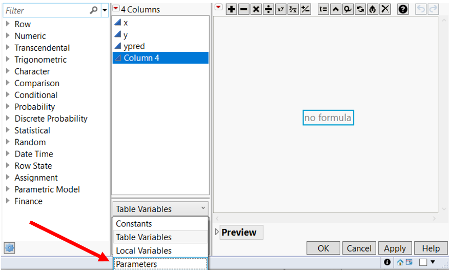Figure 1: Accessing Parameters in the Formula Editor

This brings up an option to add a "New Parameter" to the formula. Let's do a simple example and add a parameter called "a0" to the parameter list. Click on New Parameter, then change the parameter name to "a0", and give it a Value of 1:

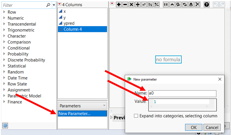Figure 2: Creating a new parameter and giving it an initial value

"Name" is arbitrary. You can choose any valid JSL variable name.
"Value" is the starting value for this parameter. You must give a starting value. Sometimes (depending on the formula that you have chosen), the starting value can be important, and should be selected to be close to the real value as you can guess. (This helps to prevent convergence problems later on.) In this case, I have no idea what the value should be, so I'll just arbitrarily choose a starting value of 1.

Now we can use this new "a0" parameter in a formula, just as if it were a column variable. Let's simply add it to the values in the column labelled "y". Double-click on a0 in the Parameter list (it should appear in the Formula panel,) then type "+", and then double-click on "y" in the column list. This should give the following formula:

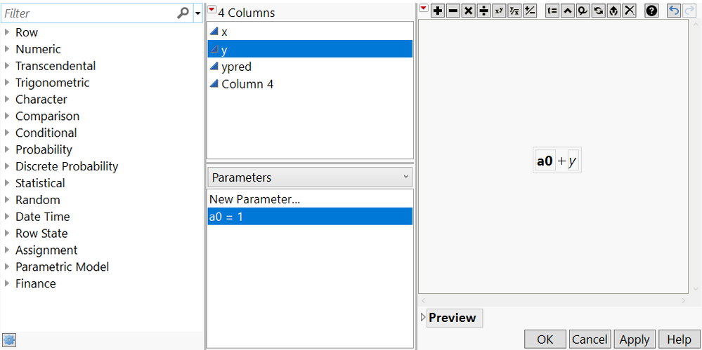Figure 3: Using a parameter in a formula

Now when we click OK and look at the result in the data table, we have

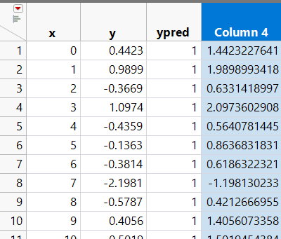Figure 4: Results of using a parameter in a formula

So the formula now recognizes the current value of the a0 parameter and applies it accordingly. This important concept will be used in the next blog post when we use the JMP Nonlinear Platform to solve for the unknown parameters.

Entering Parameters for the Piecewise Functions

In Part 2 of this blog series, we developed the five simple polynomials to apply between breakpoints in the example data series. These polynomials had six unknown parameters: a0, b1, b2, c1, d1, and d2. We also had four cutpoints defining the regions where the polynomials were active: X1, X2, X3, and X4. We need to add each of these parameters to our Formula parameter list, along with reasonable starting values. When finished, the parameter list looks like this:

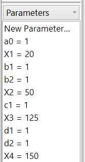Figure 5: All ten parameters entered and initialized for our piecewise example

Note that I assumed starting values of "1" for each of the coefficients in the polynomials. For the breakpoints X1 through X4, I chose to estimate values based on "eyeballing" where I thought they might occur. This simply gives JMP a better place to start looking for the breakpoints.

Entering the Piecewise Formulas - including a Boolean Trick!

Now you know how to set up parameters in the Formula Editor, and you know how to enter any of the five Piecewise equations shown in Part 2 into the Formula Editor as well. But how do we enter ALL FIVE Piecewise equations into the same formula?

One way is to use a large IF statement, e.g. "If x<X1 then (Piecewise Equation 1), else If x<X2 then (Piecewise Equation 2), etc.) This is relatively straightforward. But here I need to give a shoutout to my friend @PatrickGiuliano, who posted a helpful trick in a previous JMP Community Discussion Thread.

JMP recognizes Boolean operators (And, Or, Nor, etc.). If a Boolean operator is used in a formula, the Boolean logic returns a 1 if true, and a 0 if false. So we can set up an operator such as (X1<:x & :x<=X2). This operator returns a 1 if the value in the "x" column (referred to as ":x" in the expression) is between the parameters X1 and X2, and 0 otherwise. So we could simply multiply the piecewise equation for the X1-X2 segment by the above Boolean expression. If the value of x is in the proper range, then the segment equation is activated. If not, we return 0. We would then do the same thing for all other ranges, and sum all equations together.

If we do all of that, we end up with a formula that looks like this:

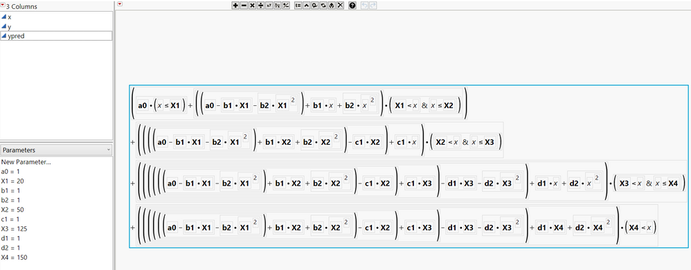Figure 6: Complete piecewise formula (shown in Formula Editor mode)

And below is the same information in JSL input format, should you prefer:

Figure 7: Complete piecewise formula (shown in JSL mode)

So to summarize, in Figures 6 and 7, we essentially have built a formula in a new column (called ypred) that:

Defines 10 unknown Parameters (and given each parameter an appropriate starting value) which will be used in the formula.
Describes four piecewise equations, each using their appropriate parameters.
Activates each piecewise equation by multiplying by an appropriate Boolean inequality that describes the ranges for each equation.
Sums the four equations to give the final formula.

Pretty cool...

Next in the series

Next time, we'll finally use the equations with the Nonlinear platform to solve for the best fit parameters. We will also discuss choices for convergence criteria and algorithms.