Wald p value not shown in JMP version 12

[#1]

I am currently using JMP 12 for my analysis . I need technical inputs on following aspect

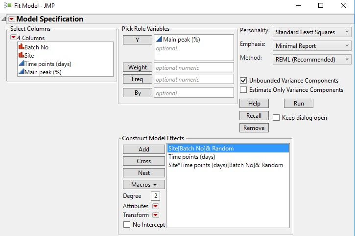
1. I am using mixed effects model  to assess whether the difference between sites is significant
2. I would like to know the wald p value corresponding to Random effect Site *time [batch] to infer whether impact is significant or not

Please let me know if there is any possibility see wald p value info in version 12 . If there is no option please let me know the formula or procedure that can be used to calculate the wald p value

Is it possible to share script for generating wald p value in JMP version 12 

Looking forward for your assistance in this regard as soon as possible as its critical for our project  

[#2]

From the JMP documentation,
Help==>Books==>Fitting Linear Models
it states for Fitting Standard Least Square models
Wald p-Value Gives the p-value for the test that the covariance parameter is equal to zero.
This column appears only when you have selected Unbounded Variance Components in
the Fit Model launch window.

[#3]

As you can see the snapshot I have shared , I am unable to get wald p value
inspite of selecting unbound variance component in fit model launch window

[#4]

Hi @Dinesh,

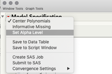
P-values are not displayed for variance components in JMP 12; these p-values were added in JMP 13. I realize it's not exactly what you're looking for, but you can use the confidence intervals in much the same way as the hypothesis test at an alpha of 1-confidence level by looking to see if 0 is contained in the interval. If it is not, your p-value (for the corresponding hypothesis test) is <  1-confidence level. If you need to change this confidence level, you can do that when you launch Fit Model: click the top red triangle in the launch window > Alpha Level.

I hope this helps some!

@julian 

[#5]

Thanks a lot Julian .That was really helpful. Is it possible to provide
script specifically to generate this wald p value . We had used used jmp
trial 14 while writing protocol and committed to include wald p value in
results .
But now we have licensed only for 12 . So to bind to that protocol , we
have to include wald p value in report . It would be of great help if you
can share the same .

Thanks a lot again for your inputs

[#6 · Accepted solution]

Hi @Dinesh,

Sure thing. That p-value is calculated with Z as the reference distribution, and the Variance Components table has all the ingredients to get the test statistic. You can save the table yourself (right click > make into data table), and then make two new columns, the ratio of the variance component to the standard error, and then a second column, a lookup of that quotient in the z-distribution, with some simple arithmetic to find the proportion more extreme than that value in the reference distribution. Here's an example of that:

Names Default To Here( 1 );
dt = Open( "$SAMPLE_DATA\Cholesterol Stacked.jmp" );

platform = dt << Fit Model(
	Y( :Y ),
	Effects(
		:Treatment,
		:Month,
		:Name( "AM/PM" ),
		:Treatment * :Month,
		:Treatment * :Name( "AM/PM" ),
		:Month * :Name( "AM/PM" ),
		:Treatment * :Month * :Name( "AM/PM" )
	),
	Random Effects(
		:Patient[:Treatment],
		:Patient * :Month[:Treatment],
		:Patient * :Name( "AM/PM" )[:Treatment],
		:Patient * :Month * :Name( "AM/PM" )[:Treatment]
	),
	NoBounds( 1 ),
	Personality( "Standard Least Squares" ),
	Method( "REML" ),
	Emphasis( "Minimal Report" ),
	Run(
		:Y << {Summary of Fit( 1 ), Analysis of Variance( 0 ), Parameter Estimates( 1 ), Lack of Fit( 0 ),
		Scaled Estimates( 0 ), Plot Actual by Predicted( 0 ), Plot Regression( 0 ),
		Plot Residual by Predicted( 0 ), Plot Studentized Residuals( 0 ), Plot Effect Leverage( 0 ),
		Plot Residual by Normal Quantiles( 0 )}
	)
);

Wait( 0 );
Report( platform )[Outline Box( "Response Y" )][Outline Box( "REML Variance Component Estimates" )][
Table Box( 1 )] << Make Into Data Table;
Report( platform ) << Close Window;



New Column( "Var Component/Std Error",
	Numeric,
	"Continuous",
	Format( "Best", 12 ),
	Formula( :Var Component / :Std Error ),
	Set Selected
);
New Column( "Prob > |Z|",
	Numeric,
	"Continuous",
	Format( "Best", 12 ),
	Formula( (1 - Normal Distribution( :Name( "Var Component/Std Error" ) )) * 2 ),
	Set Selected
);

This will return the following (showing JMP 14 so you can see JMP's calculation of the Wald P-value, which you can confirm is the same as the one calculated in the method I described above).

@julian