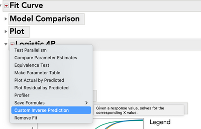
Go to this menu: Analyze>Specialized Modeling>Fit Curve.
Put in your X, Y and Group variables.
Try fitting Sigmoidal Curve, 4p Logistic, or a model like that.
After you fit the model, look under the red triangle menu for the fit to find inverse prediction:

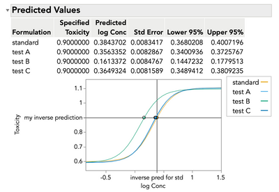
Here's an example using the sample data of what it will look like:

Note: I added the reference line annotations, those don't happen automatically .
Names Default To Here( 1 );
dt = Open( "$SAMPLE_DATA/Nonlinear Examples/Bioassay.jmp" );

Fit Curve(
	Y( :Toxicity ),
	X( :log Conc ),
	Group( :Formulation ),
	Fit Logistic 4P( Custom Inverse Prediction( Response( 0.9 ) ) ),
	SendToReport(
		Dispatch( {}, "Model Comparison", OutlineBox, {Close( 1 )} ),
		Dispatch( {}, "Plot", OutlineBox, {Close( 1 )} ),
		Dispatch( {"Logistic 4P"}, "Group Summary", OutlineBox, {Close( 1 )} ),
		Dispatch(
			{"Logistic 4P", "Inverse Prediction", "Predicted Values"},
			"1",
			ScaleBox,
			{Add Ref Line( 0.3843702, "Solid", "Black", "inverse pred for std", 1 )}
		),
		Dispatch(
			{"Logistic 4P", "Inverse Prediction", "Predicted Values"},
			"2",
			ScaleBox,
			{Add Ref Line( 0.9, "Solid", "Black", "my inverse prediction", 1 )}
		)
	)
);
JMP Systems Engineer, Health and Life Sciences (Pharma)