- New to JMP? Let the Data Analysis Director guide you through selecting an analysis task, an analysis goal, and a data type. Available now in the JMP Marketplace!
- See how to install JMP Marketplace extensions to customize and enhance JMP.
- Subscribe to RSS Feed
- Mark Topic as New
- Mark Topic as Read
- Float this Topic for Current User
- Bookmark
- Subscribe
- Mute
- Printer Friendly Page
Discussions
Solve problems, and share tips and tricks with other JMP users.- JMP User Community
- :
- Discussions
- :
- Re: Probit Analysis & Fit Testing
- Mark as New
- Bookmark
- Subscribe
- Mute
- Subscribe to RSS Feed
- Get Direct Link
- Report Inappropriate Content
Probit Analysis & Fit Testing
I am using the Simple Probit Analysis script add-in to determine LD50, LD90, and LD95.
Is this script capable of correcting with Abbott's, or how do you set this up? Currently, I corrected the data myself by applying the Abbott's correction to the raw data to adjust for mortalities.
After running the Probit Add-In, how do I determine goodness of fit? There are no Chi Squared results. Is there another way I can run this analysis to get my LD values, as well as getting the Chi Square?
- Mark as New
- Bookmark
- Subscribe
- Mute
- Subscribe to RSS Feed
- Get Direct Link
- Report Inappropriate Content
Re: Probit Analysis & Fit Testing
Your last comment about testing mortality rates over time changes everything, I think. My example is not relevant. My example is a case where a number of samples or subjects (20) is assigned to each factor level (5). Each level is an independent sample (5x20). The total number of samples or subjects is the sum of the samples at each level (100). I believe that you start with a fixed number of subjects (e.g. 60 total), the agent level is introduced at a fixed level, and you monitor the same group (subjects) over time. Yes?
Assuming I am correct, then you want to use repeated measures in survival analysis.
The methods and platforms in JMP were developed for reliability analysis, but it is the same thing. Just be warned that the words and labels are for reliability engineers and not biologists, if you know what I mean.
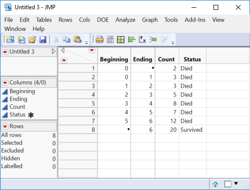
Set up your data to look like this example:
In this example, I have a total of 60 subjects that I monitor from the start of a 6 month program. I need two columns to represent the response (life) because I am not monitoring the subjects continuously but at monthly intervals. This process leads to interval censoring. I don't observe the exact life but instead I observe that it occurs during an interval.
- The first row represents the start of the test. In this simulation, 2 subjects died at the start.
- The second row represents the number of subjects who died between the start and the end of the first month (3).
- The third row represents the number of subjects who died in the second month (3), and so on.
- The last row represents the number of subjects who did not die by the end of the study (20).
I added another column, Status, to indicate the status of the observations but it is not necessary for the analysis. Perform the analyis by following these steps:
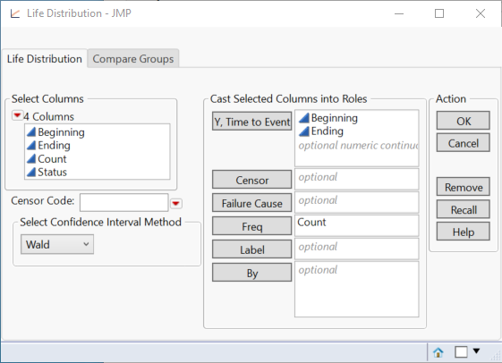
- Select Analyze > Reliability and Survival > Life Distribution.
- Select Beginning and Ending and click Y, Time to Event.
- Select Count and click Freq.
The launch dialog should look like this:
(Note that the Censor analysis role is for right censored data. It is not needed when two response columns are used for interval censoring.)
Click OK.
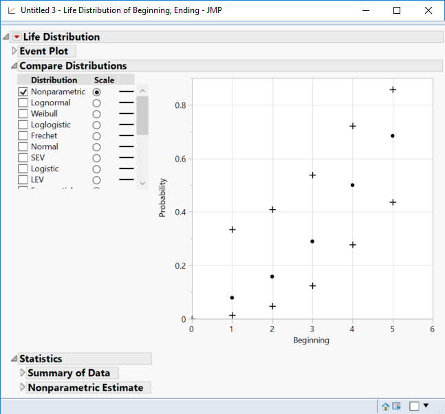
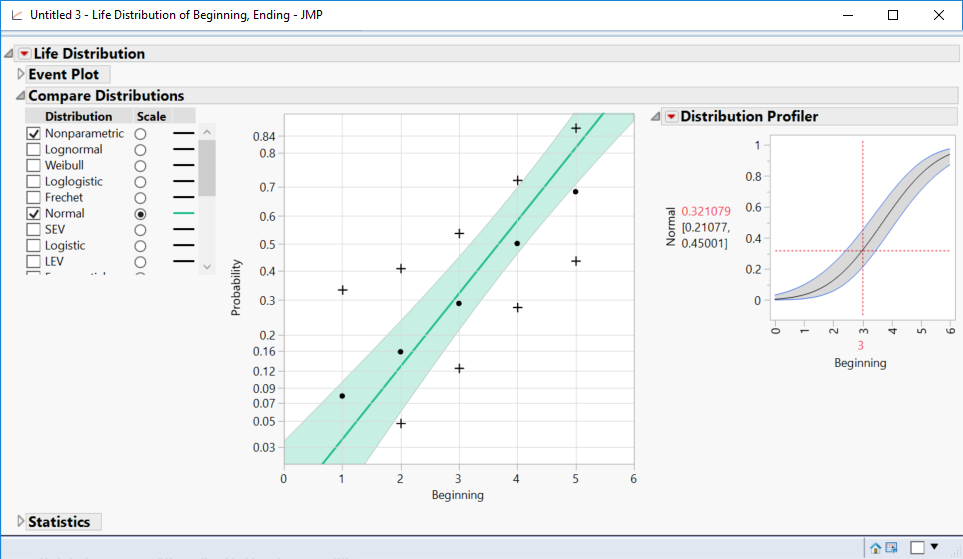
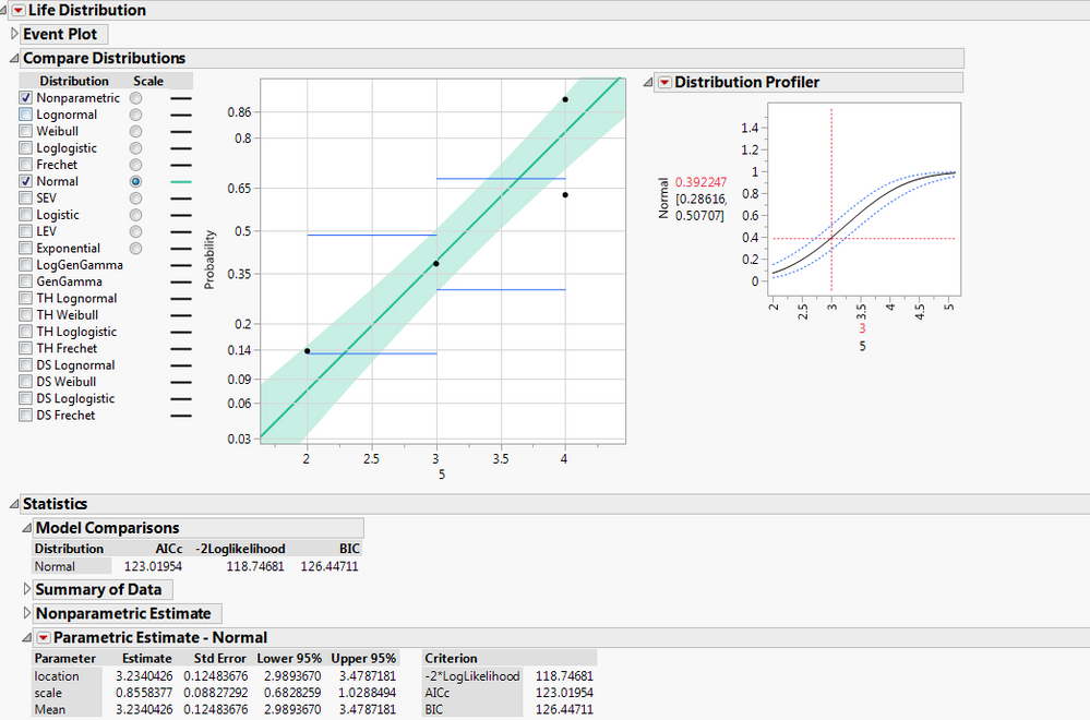
The initial analysis is based on the non-parametric estimates of the failure probability from the Kaplan-Meier product limit. (You can click the red triangle at the top to change it from a Failure plot to a Survival plot.) You use the check boxes and radio buttons on the left side to scale the plot and fit a distribution model, respectively, to the data. Let's fit a normal distribution. Check the Normal check box and click the Normal radio button:
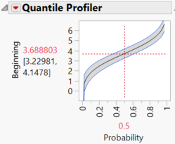
After selecting a model, use the Statistics outline to obtain the desired results. For example, your LD50 is available here as the quantile corresponding to a failure probability = 0.5, so estimate LD50 with the Quantile Profiler:
The LD50 in this example is 3.688803 months (3.22981 months to 4.1478 months with 95% confidence).
- Mark as New
- Bookmark
- Subscribe
- Mute
- Subscribe to RSS Feed
- Get Direct Link
- Report Inappropriate Content
Re: Probit Analysis & Fit Testing
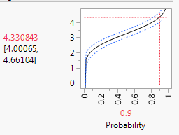
So I used my raw, unadjusted data without my controls and came up with this.
Do I interpret this as: LD90 for 100% Dose is 4.33 minutes? How do I determine the fit of this since there is no Chi Square? (I'm being asked to show a goodness of fit for the model I use.)
Do I count mortality as a "failure"?
- Mark as New
- Bookmark
- Subscribe
- Mute
- Subscribe to RSS Feed
- Get Direct Link
- Report Inappropriate Content
Re: Probit Analysis & Fit Testing
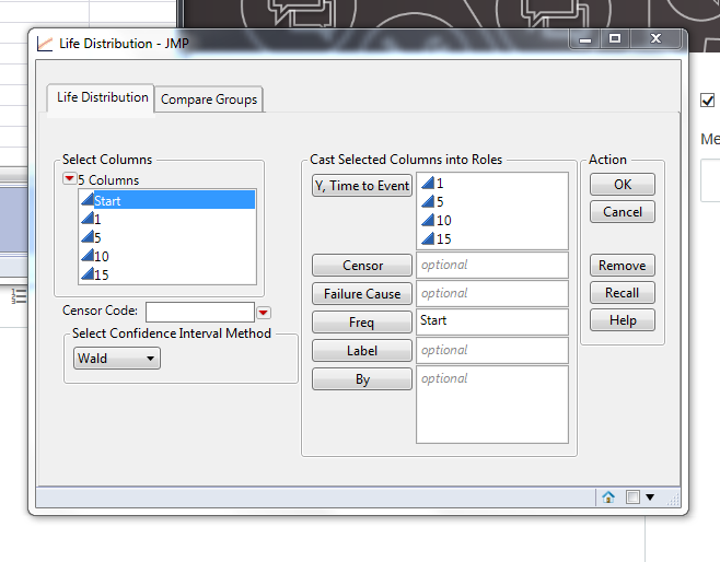
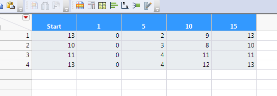
Here's how I set it up and my data:
- Mark as New
- Bookmark
- Subscribe
- Mute
- Subscribe to RSS Feed
- Get Direct Link
- Report Inappropriate Content
Re: Probit Analysis & Fit Testing
I'm not sure that is going to work. I'm getting resistence from others around me on running the analysis that way. They want the probit.
- Mark as New
- Bookmark
- Subscribe
- Mute
- Subscribe to RSS Feed
- Get Direct Link
- Report Inappropriate Content
Re: Probit Analysis & Fit Testing
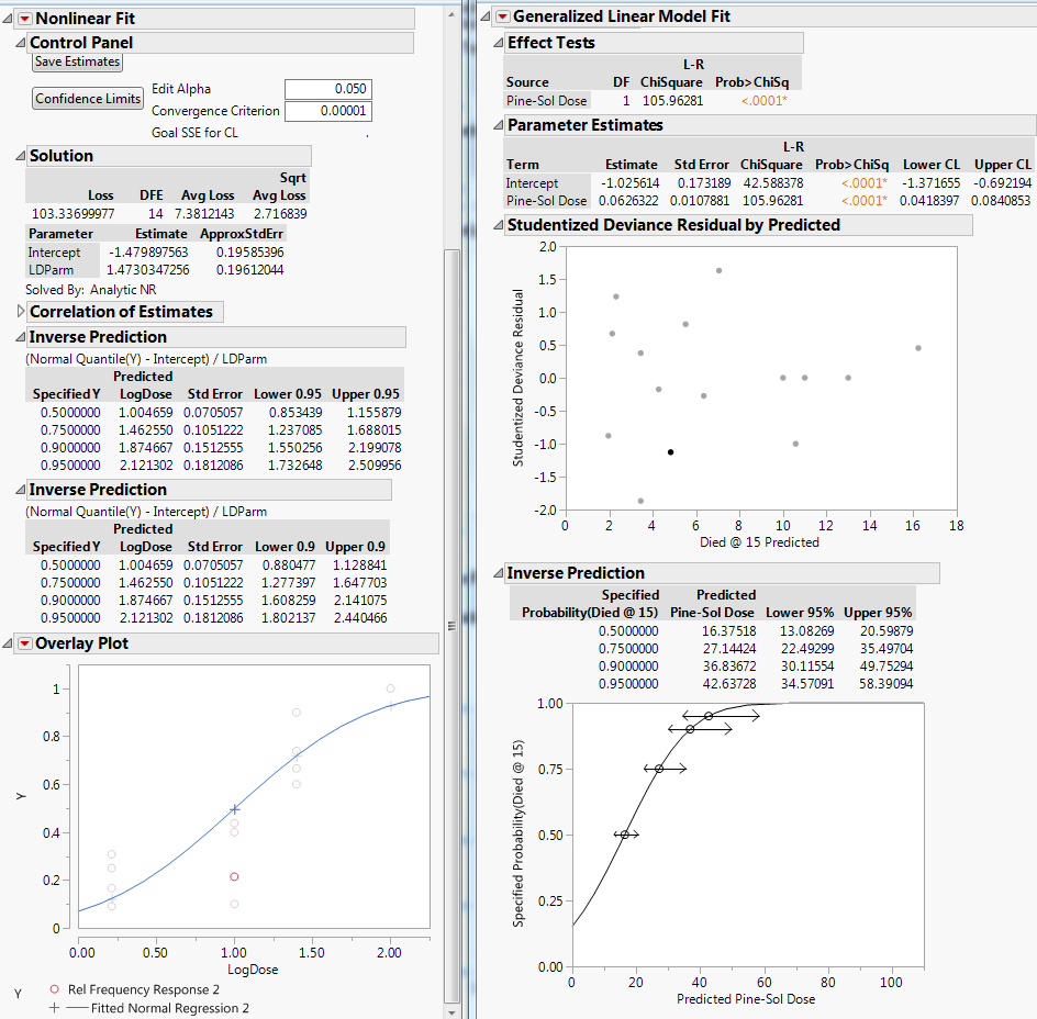
Here is the comparison of the same data in the probit add in vs the gen. linear probit. If I revert predicted log dose back, it does not match up with the same results in the general linear model.
- Mark as New
- Bookmark
- Subscribe
- Mute
- Subscribe to RSS Feed
- Get Direct Link
- Report Inappropriate Content
Re: Probit Analysis & Fit Testing
So if I run the GLM, do I include my controls/0 doses?
- Mark as New
- Bookmark
- Subscribe
- Mute
- Subscribe to RSS Feed
- Get Direct Link
- Report Inappropriate Content
Re: Probit Analysis & Fit Testing
I apologize (though it is not my fault) for the replies getting out of order. It does not help the confusion that already exists.
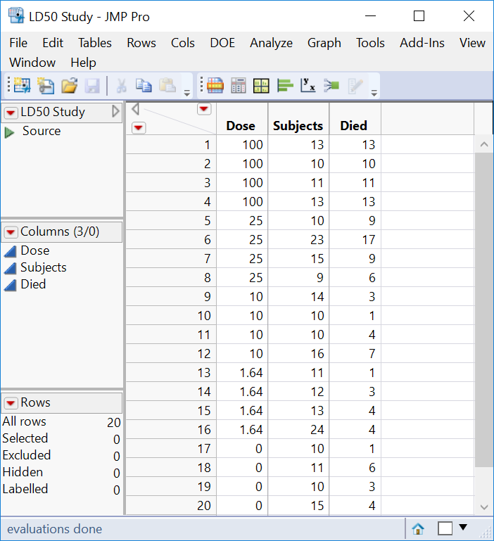
I have one question before I think we can conclude this discussion: why do you have four observations (rows) for each dose? What does each row represent?
Again, forget Life Distribution. Your colleagues are correct, you need a probit analysis. I am working now to make sure that your data table is set up correctly and the analysis is properly defined in Fit Model for a probit analysis. I want to use your previous example of data after you explain why there are four rows for every dose:
- Mark as New
- Bookmark
- Subscribe
- Mute
- Subscribe to RSS Feed
- Get Direct Link
- Report Inappropriate Content
Re: Probit Analysis & Fit Testing
I have 4 rows because I performed 4 replicates at each dose. I had 4 doses, 4 reps each. I did monitor each treatment at 1 min, 5 min, 10 min, and 15 min intervals.
- Mark as New
- Bookmark
- Subscribe
- Mute
- Subscribe to RSS Feed
- Get Direct Link
- Report Inappropriate Content
Re: Probit Analysis & Fit Testing
- Mark as New
- Bookmark
- Subscribe
- Mute
- Subscribe to RSS Feed
- Get Direct Link
- Report Inappropriate Content
Re: Probit Analysis & Fit Testing
Yes, you include the control group with dose = 0.
You enter both counts for each dose, so you do not use mortality rate and you do not apply Abbott's correction.
You should perform a separate Probit analysis for each time interval. I performed the correct Probit analysis for the dose-response data collected after 15 minutes already (shown above - the reply with the correct analysis ends with my question for you, "So we agree now, no?"). Let me know if you have any questions.
Perform this analysis for the data collected after the other intervals. Let me know if you have trouble repeating this work.
You should not expect the estimates to be the same for each group (collection time). You should perform the analysis correctly and not compare the results to those from other variations that are not correct.
Recommended Articles
- © 2026 JMP Statistical Discovery LLC. All Rights Reserved.
- Terms of Use
- Privacy Statement
- Contact Us

