- New to JMP? Let the Data Analysis Director guide you through selecting an analysis task, an analysis goal, and a data type. Available now in the JMP Marketplace!
- See how to install JMP Marketplace extensions to customize and enhance JMP.
- Subscribe to RSS Feed
- Mark Topic as New
- Mark Topic as Read
- Float this Topic for Current User
- Bookmark
- Subscribe
- Mute
- Printer Friendly Page
Discussions
Solve problems, and share tips and tricks with other JMP users.- JMP User Community
- :
- Discussions
- :
- Re: How do I generate an AUC p value
- Mark as New
- Bookmark
- Subscribe
- Mute
- Subscribe to RSS Feed
- Get Direct Link
- Report Inappropriate Content
How do I generate an AUC p value
When running a logistic regression I do get the whole model fit p value. nevertheless in many papers I read they report on p values of the AUC speicificaly, and from my understanding this is a p-value that tests the null hypothesis that the area under the curve really equals 0.50. It seems that other softwares do provide this by default. I would appreciate your suggestion on this matter.
Accepted Solutions
- Mark as New
- Bookmark
- Subscribe
- Mute
- Subscribe to RSS Feed
- Get Direct Link
- Report Inappropriate Content
Re: How do I generate an AUC p value
Hi @eliyahu100,
(TLDR: bootstrapping and randomization testing can be used, in different ways, to get at an empirical p-value for AUCroc, and through these we can see why the p-value for AUCroc ends up being the whole model test).
My first impression is that any p-value one might obtain from a test of the AUCroc is conceptually equivalent to the whole model test of the classifier (whether that be logistic regression or otherwise). That is, testing whether there is evidence that AUCroc is different from what would be expected under the null hypothesis (random classification) appears tantamount to whether a model explains more error (i.e. classifies) than would be expected by chance alone. That said, I was able to find various methods describing how one could calculate an AUCroc p-value (e.g. Hajian-Tilaki, 2013), and we can safely say JMP does not perform these calculations by default (though anything is possible via scripting, of course). Looking through these formulae got me wondering, however, about the performance of these hypothesis tests and the assumptions they make. If you have access to JMP Pro, there is something you can do right this minute that will likely outperform the large sample/normal approximation formulas used to obtain p-values for AUCroc, and that's bootstrapping and/or simulation/randomization test. Here's how we'd do it:
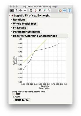
1. Fit a classifier model. I'll be using Big Class, and will predict sex by height. Reveal the AUCroc from the Red Triangle.
Open("$SAMPLE_DATA\Big Class.jmp");
Logistic(Y( :sex ),X( :height ), Positive Level( "M" ),
	Logistic Plot( 0 ), ROC Curve( 1 ),
	SendToReport(
		Dispatch( {}, "Whole Model Test", OutlineBox, {Close( 1 )} ),
		Dispatch( {}, "Parameter Estimates", OutlineBox, {Close( 1 )} )
	));
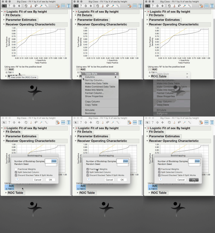
2. First, let's try with Bootstrapping. Right-click the reported AUCroc value, then select Bootstrap. Use at least 2500 bootstrap samples, and I like fractional weights, especially if you have any categories that have low relative frequencies.
This will return a table of bootstrapped AUCroc values -- what you get from sampling with replacement from your table and recalculating the model and AUCroc, storing at each iteration the value you get. In essence, you now have the sampling distribution of AUCroc for your given classifier. Obtaining a p-value is now just a matter of counting. But, let's let JMP do that.
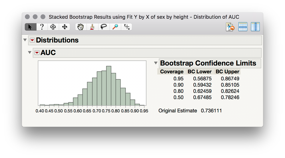
3. Analyze > Distribution, then put AUC as Y, and check "Histograms only," then click OK:
You now have the bootstrap confidence limits on AUCroc, which are great for reporting, plus if you wish to know whether your originally obtained AUCroc is different from a particular value, you just need to see whether that null value is within the confidence interval at your chosen level of confidence.
But, you asked for a p-value. We could literally count how many times out of the 2500 samples we obtained an AUCroc at 0.50 or less, but we can do one better. JMP is adding special output to this distribution report because there is a BootID column in your table. JMP knows how to work with that column in conjunction with the first row in your table (the original sample estimate). If we wanted, we can change things around to make this a kind of randomization test rather than a bootstrap (and we'll do the proper randomization test later on to compare). We just need to make two simple changes: Rename the column "BootID•" to "SimID•" and change the value of the original estimate in the table to the value you wish to test against... that is, change the value in the first row of the AUC column to 0.50. Here's what the top of your table should now look like:
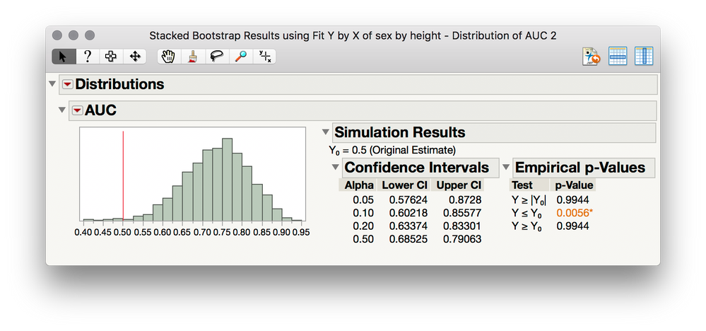
Now launch Analyze > Distribution, again put AUC in for Y, and check Histrograms only. We will get the following output:
Notice that JMP is presenting us with "Simulation Results" rather than bootstrap results. This is due to the change of the BootID column (SimID is what right-click simulate provides). We're finagling things a bit here so know that this isn't typically how JMP reports simulation results (we'll see how it works normally next), but in this case JMP has drawn a line for where you placed your null hypothesis value of AUCroc (0.50), and in your p-value of Y<=Y0 you can see the proportion of time you obtained a random sample (from your original data) with an AUCroc less than or equal to 0.50. This is your empirical one tailed p-value, given 0.50 as your null. But, let's not stop here since another approach to this can yield something interesting and important.
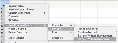
Another way (and frankly, the better way) we could have gone about this if an empirical p-value is our desired outcome, is using Right Click > Simulate on the reported AUCroc. Much like Bootstrapping, we will involve resampling with replacement from our table (or without replacement if we wish to do a permutation test). In order to do this as a Right Click > Simulate, we need to create a new formula column for the simulator that will handle the sampling with replacement. A simple way to do this is to select the Y column in your table, right-click the header row > New Formula Column > Random > Sample with Replacement.
This makes a new column (Resample[sex]), and every time the formula for this column is rereun the labels of M and F are randomly assigned to the table based on the observed base rates (i.e., sampling with replacement).
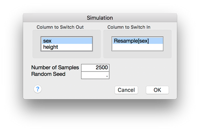
Next, let's return to our logistic regression and right-click AUCroc in the report, but rather than select Bootstrap, we select Simulate. We will be prompted to pick a formula column to substitute for a column used in our report. In this case, I would select sex and Resample[sex]. Do at least 2500 samples, but for this example, I'll do 10k just so we get a more precise estimate of the resulting statistics.
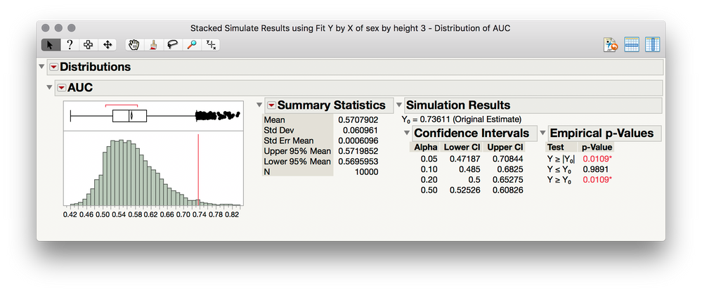
After JMP finishes we are given a very similar table to the bootstrap, but what we have now is not the sampling distribution of AUCroc given our original data, but the sampling distribution of AUCroc given no relation between sex and height but honoring the base rates of sex (since we are simulating what would happen if we were randomly assigning the labels of M and F to rows in our table -- this is the null hypothesis). I'll choose Analyze > Distribution, place AUC in for Y, but this time let's not check the box for Histograms only because there is something important to notice here:
Our empirical p-values are reported again, but this time our estimates of AUCroc hover toward 0.50 (but not actually 0.50, we'll come back to why) whereas from the bootstrap they hovered around our observed estimate. Again, in this case, we're simulating what happens to AUCroc under the null hypothesis, so this should make sense. The empirical p-values here then are reporting how often we obtain estimates from this sampling distribution that exceed our original estimate (which is our typical definition of a p-value: how unlikely is our estimate given chance alone is responsible for the generation of the values). Two things to notice here:
1. Our empirical p-value is 0.0190, which is identical to the p-value from the original whole model test.
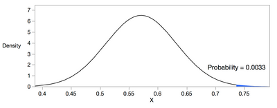
2. Notice that the sampling distribution here does not have a mean of 0.50. That is, the expected value here is not 0.50 and so the empirical p-values given are not with regard to a null of 0.50, but rather a null of, in this case, about 0.57. This is due to the proportion of males and females in this dataset -- if we're just guessing randomly with respect to height, but know there are more males than females, we can guess male more often and do better than 50% classification accuracy (our model intercept accounts for this). Side note: notice that this sampling distribution is decidedly non-normal, and yet p-values obtained from large sample approximation formulae (like the one I referenced at the start) would have you believe this sampling distribution is normal. If we simply use the mean and standard deviation and perform a p-value lookup that way, we get p = 0.0033, not p = 0.0190. That's a big difference, and a great reason why randomization tests are great: no assumptions about distributional shape.
One more point: the differences between the bootstrap and randomization test are important, even though they can provide what seems like similar information. In the bootstrap we changed the BootID column to be SimID to hack JMP to give us the empirical p-value report, and changed a value in the table to set the null AUCroc to exactly 0.50. What we got is an empirical p-value, but we went about it from the perspective of the sample estimate (in the way a confidence interval is from the perspective of the sample estimate). For the randomization test via right-click Simulate, we take the perspective of the null, and we allowed jmp to generate the sampling distribution under the null hypothesis for AUCroc and then compared our original estimate to that. Neither of these is more accurate, but they do end up giving you subtly different things and it's good to understand both.
The biggest difference, however, it not the conceptual difference of statistical perspective each approach takes, it's the specification of 0.50 as the null in our bootstrap variant. You might be wondering, what if we used the bootstrap table and set the null hypothesis value to the value under the null we obtained from the randomization test (0.57079)?
Well, if you're a believer, like me, in the randomness of randomness being a certainty, you should be expecting our empirical p-value generated from bootstrapped samples against the same null to be pretty similar to the actual randomization test. After all, aren't they estimating the same thing conceptually, just from different perspectives?
Well look at that, p = 0.0192. Faith in randomness upheld. :)
I do hope this helps some!
- Mark as New
- Bookmark
- Subscribe
- Mute
- Subscribe to RSS Feed
- Get Direct Link
- Report Inappropriate Content
Re: How do I generate an AUC p value
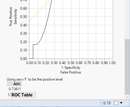
The Statistics Index has an example of how to do this. If you are not familiar with the Statistics Index, it is available at:
Help==>Statistics Index
Here is the example taken from the index entry
Names Default To Here( 1 );
Open(
	"$SAMPLE_DATA/Big Class.jmp"
);
Logistic(
	Y( :sex ),
	X( :height ),
	Positive Level( "F" ),
	ROC Curve
);- Mark as New
- Bookmark
- Subscribe
- Mute
- Subscribe to RSS Feed
- Get Direct Link
- Report Inappropriate Content
Re: How do I generate an AUC p value
I think the question is not how to get the AUC but how to determine a p value for whether it is significantly different from 0.5. While I'm not a big fan of p-values, I'd like to know the answer as well. It does appear that there is a test that provides this, but I don't see anywhere in JMP to obtain that.
- Mark as New
- Bookmark
- Subscribe
- Mute
- Subscribe to RSS Feed
- Get Direct Link
- Report Inappropriate Content
Re: How do I generate an AUC p value
Indeed my question was regarding the p-value and this is still not solved. any help would be appriciated.
@dale_lehman wrote:I think the question is not how to get the AUC but how to determine a p value for whether it is significantly different from 0.5. While I'm not a big fan of p-values, I'd like to know the answer as well. It does appear that there is a test that provides this, but I don't see anywhere in JMP to obtain that.
- Mark as New
- Bookmark
- Subscribe
- Mute
- Subscribe to RSS Feed
- Get Direct Link
- Report Inappropriate Content
Re: How do I generate an AUC p value
Hi @eliyahu100,
(TLDR: bootstrapping and randomization testing can be used, in different ways, to get at an empirical p-value for AUCroc, and through these we can see why the p-value for AUCroc ends up being the whole model test).
My first impression is that any p-value one might obtain from a test of the AUCroc is conceptually equivalent to the whole model test of the classifier (whether that be logistic regression or otherwise). That is, testing whether there is evidence that AUCroc is different from what would be expected under the null hypothesis (random classification) appears tantamount to whether a model explains more error (i.e. classifies) than would be expected by chance alone. That said, I was able to find various methods describing how one could calculate an AUCroc p-value (e.g. Hajian-Tilaki, 2013), and we can safely say JMP does not perform these calculations by default (though anything is possible via scripting, of course). Looking through these formulae got me wondering, however, about the performance of these hypothesis tests and the assumptions they make. If you have access to JMP Pro, there is something you can do right this minute that will likely outperform the large sample/normal approximation formulas used to obtain p-values for AUCroc, and that's bootstrapping and/or simulation/randomization test. Here's how we'd do it:
1. Fit a classifier model. I'll be using Big Class, and will predict sex by height. Reveal the AUCroc from the Red Triangle.
Open("$SAMPLE_DATA\Big Class.jmp");
Logistic(Y( :sex ),X( :height ), Positive Level( "M" ),
	Logistic Plot( 0 ), ROC Curve( 1 ),
	SendToReport(
		Dispatch( {}, "Whole Model Test", OutlineBox, {Close( 1 )} ),
		Dispatch( {}, "Parameter Estimates", OutlineBox, {Close( 1 )} )
	));
2. First, let's try with Bootstrapping. Right-click the reported AUCroc value, then select Bootstrap. Use at least 2500 bootstrap samples, and I like fractional weights, especially if you have any categories that have low relative frequencies.
This will return a table of bootstrapped AUCroc values -- what you get from sampling with replacement from your table and recalculating the model and AUCroc, storing at each iteration the value you get. In essence, you now have the sampling distribution of AUCroc for your given classifier. Obtaining a p-value is now just a matter of counting. But, let's let JMP do that.
3. Analyze > Distribution, then put AUC as Y, and check "Histograms only," then click OK:
You now have the bootstrap confidence limits on AUCroc, which are great for reporting, plus if you wish to know whether your originally obtained AUCroc is different from a particular value, you just need to see whether that null value is within the confidence interval at your chosen level of confidence.
But, you asked for a p-value. We could literally count how many times out of the 2500 samples we obtained an AUCroc at 0.50 or less, but we can do one better. JMP is adding special output to this distribution report because there is a BootID column in your table. JMP knows how to work with that column in conjunction with the first row in your table (the original sample estimate). If we wanted, we can change things around to make this a kind of randomization test rather than a bootstrap (and we'll do the proper randomization test later on to compare). We just need to make two simple changes: Rename the column "BootID•" to "SimID•" and change the value of the original estimate in the table to the value you wish to test against... that is, change the value in the first row of the AUC column to 0.50. Here's what the top of your table should now look like:
Now launch Analyze > Distribution, again put AUC in for Y, and check Histrograms only. We will get the following output:
Notice that JMP is presenting us with "Simulation Results" rather than bootstrap results. This is due to the change of the BootID column (SimID is what right-click simulate provides). We're finagling things a bit here so know that this isn't typically how JMP reports simulation results (we'll see how it works normally next), but in this case JMP has drawn a line for where you placed your null hypothesis value of AUCroc (0.50), and in your p-value of Y<=Y0 you can see the proportion of time you obtained a random sample (from your original data) with an AUCroc less than or equal to 0.50. This is your empirical one tailed p-value, given 0.50 as your null. But, let's not stop here since another approach to this can yield something interesting and important.
Another way (and frankly, the better way) we could have gone about this if an empirical p-value is our desired outcome, is using Right Click > Simulate on the reported AUCroc. Much like Bootstrapping, we will involve resampling with replacement from our table (or without replacement if we wish to do a permutation test). In order to do this as a Right Click > Simulate, we need to create a new formula column for the simulator that will handle the sampling with replacement. A simple way to do this is to select the Y column in your table, right-click the header row > New Formula Column > Random > Sample with Replacement.
This makes a new column (Resample[sex]), and every time the formula for this column is rereun the labels of M and F are randomly assigned to the table based on the observed base rates (i.e., sampling with replacement).
Next, let's return to our logistic regression and right-click AUCroc in the report, but rather than select Bootstrap, we select Simulate. We will be prompted to pick a formula column to substitute for a column used in our report. In this case, I would select sex and Resample[sex]. Do at least 2500 samples, but for this example, I'll do 10k just so we get a more precise estimate of the resulting statistics.
After JMP finishes we are given a very similar table to the bootstrap, but what we have now is not the sampling distribution of AUCroc given our original data, but the sampling distribution of AUCroc given no relation between sex and height but honoring the base rates of sex (since we are simulating what would happen if we were randomly assigning the labels of M and F to rows in our table -- this is the null hypothesis). I'll choose Analyze > Distribution, place AUC in for Y, but this time let's not check the box for Histograms only because there is something important to notice here:
Our empirical p-values are reported again, but this time our estimates of AUCroc hover toward 0.50 (but not actually 0.50, we'll come back to why) whereas from the bootstrap they hovered around our observed estimate. Again, in this case, we're simulating what happens to AUCroc under the null hypothesis, so this should make sense. The empirical p-values here then are reporting how often we obtain estimates from this sampling distribution that exceed our original estimate (which is our typical definition of a p-value: how unlikely is our estimate given chance alone is responsible for the generation of the values). Two things to notice here:
1. Our empirical p-value is 0.0190, which is identical to the p-value from the original whole model test.
2. Notice that the sampling distribution here does not have a mean of 0.50. That is, the expected value here is not 0.50 and so the empirical p-values given are not with regard to a null of 0.50, but rather a null of, in this case, about 0.57. This is due to the proportion of males and females in this dataset -- if we're just guessing randomly with respect to height, but know there are more males than females, we can guess male more often and do better than 50% classification accuracy (our model intercept accounts for this). Side note: notice that this sampling distribution is decidedly non-normal, and yet p-values obtained from large sample approximation formulae (like the one I referenced at the start) would have you believe this sampling distribution is normal. If we simply use the mean and standard deviation and perform a p-value lookup that way, we get p = 0.0033, not p = 0.0190. That's a big difference, and a great reason why randomization tests are great: no assumptions about distributional shape.
One more point: the differences between the bootstrap and randomization test are important, even though they can provide what seems like similar information. In the bootstrap we changed the BootID column to be SimID to hack JMP to give us the empirical p-value report, and changed a value in the table to set the null AUCroc to exactly 0.50. What we got is an empirical p-value, but we went about it from the perspective of the sample estimate (in the way a confidence interval is from the perspective of the sample estimate). For the randomization test via right-click Simulate, we take the perspective of the null, and we allowed jmp to generate the sampling distribution under the null hypothesis for AUCroc and then compared our original estimate to that. Neither of these is more accurate, but they do end up giving you subtly different things and it's good to understand both.
The biggest difference, however, it not the conceptual difference of statistical perspective each approach takes, it's the specification of 0.50 as the null in our bootstrap variant. You might be wondering, what if we used the bootstrap table and set the null hypothesis value to the value under the null we obtained from the randomization test (0.57079)?
Well, if you're a believer, like me, in the randomness of randomness being a certainty, you should be expecting our empirical p-value generated from bootstrapped samples against the same null to be pretty similar to the actual randomization test. After all, aren't they estimating the same thing conceptually, just from different perspectives?
Well look at that, p = 0.0192. Faith in randomness upheld. :)
I do hope this helps some!
Recommended Articles
- © 2026 JMP Statistical Discovery LLC. All Rights Reserved.
- Terms of Use
- Privacy Statement
- Contact Us

