- Subscribe to RSS Feed
- Mark Topic as New
- Mark Topic as Read
- Float this Topic for Current User
- Bookmark
- Subscribe
- Mute
- Printer Friendly Page
Discussions
Solve problems, and share tips and tricks with other JMP users.- JMP User Community
- :
- Discussions
- :
- Re: How can use JMP to decompose a curve into an original three-condition curve?
- Mark as New
- Bookmark
- Subscribe
- Mute
- Subscribe to RSS Feed
- Get Direct Link
- Report Inappropriate Content
How can use JMP to decompose a curve into an original three-condition curve?
Hello, everyone!
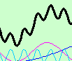
The Y curve is the sum of the other three curves.
Specific formula is: Y = Max + mid + min + 10
If only know Y, I need to restore the three curves of "Max", "mid" and "min".
I've looked it up and it looks like I can do it with the Fourier transform.
I would like to ask if there is a corresponding module with JMP to achieve this restore.

The excel formula of the other three curves is:
min=ROUND(2*SIN(80*RADIANS(:x)+RADIANS(7)),10)+2
mid=ROUND(3*SIN(21*RADIANS(:x)+RADIANS(8)),10)+3
max=ROUND(4*SIN(5*RADIANS(:x)+RADIANS(64)),10)+4
Thanks!
Accepted Solutions

- Mark as New
- Bookmark
- Subscribe
- Mute
- Subscribe to RSS Feed
- Get Direct Link
- Report Inappropriate Content
Re: How can use JMP to decompose a curve into an original three-condition curve?
What are you hoping to recover?
- Frequency/Amplitude
- Phase
- DC offset
Recovering the three frequency and amplitude components (80,21,5 and 2,3,4) is easy with the FFT function, though real world data adds complications. See FFT and DTMF for an old example. Recovering the phase seems hard. My experiment below recovers (7,8,64) if the buffer length perfectly matches the wave form's period, otherwise I think the phase information may be lost. (I'm not an expert on this subject.) Recovering the individual DC offsets is impossible because they are all added together.
This JSL needs lots more testing before you put it to use!
RADIANS = Function( {x}, 2 * Pi() * x / 360 );

NSAMPLES = 360; // 360 makes the answer look perfect. Real-world data will change everything for the worse...
time = NSAMPLES/360; // number of seconds the table holds

dt = New Table( "Untitled 4",
	Add Rows( NSAMPLES ),// generate perfect, non-real world data
	New Column( "x", formula( Row()-1 ) ), // time axis, in degrees
	// not sure why you would round this to 10 places, but it was part of the question...
	// adding 7 degrees is a phase adjustment, multiplying by 2 is an amplitude adjustment
	// adding 2+3+4 at the end is the DC level of 9. You'll never get those individual values back, just the 9.
	New Column( "min", formula( Round( 2 * Sin( 80/*Hz*/ * RADIANS( :x ) + RADIANS( 7/*degrees*/ ) ), 10 ) + 2 ) ),
	New Column( "mid", formula( Round( 3 * Sin( 21/*Hz*/ * RADIANS( :x ) + RADIANS( 8/*degrees*/ ) ), 10 ) + 3 ) ),
	New Column( "max", formula( Round( 4 * Sin( 5/*Hz*/ * RADIANS( :x ) + RADIANS( 64/*degrees*/ ) ), 10 ) + 4 ) ),
	New Column( "combine", formula( min + mid + max ) )
);
dt << Graph Builder( Size( 1275, 240 ), Show Control Panel( 0 ), Variables( X( :x ), Y( :combine ) ), Elements( Line( X, Y, Legend( 11 ) ) ),
	SendToReport( Dispatch( {}, "graph title", TextEditBox, {Set Text( "Original Data" )} ) ) );

// there are NSAMPLES and there will be NSAMPLES bins in the FFT result.
// the first half of the bins are interesting, 1..(NSAMPLES/2), the 2nd half mirror them.
// the lowest bin, 1, will represent the DC offset
// The bins 1-(NSAMPLES/2) are equal width in frequency; the maximum frequency is
// NSAMPLES/2 full cycles in a buffer (or (NSAMPLES/2) radians per buffer)
// (you know how much time a buffer represents, so you can get back to Hz)

freq = (((1 :: (NSAMPLES / 2)) - 1) / time)`; // cycles per second for each bin

{real, complex} = FFT( {dt[0, "combine"]} );
amplitude = Sqrt( real ^ 2 + complex ^ 2 );
dt2 = As Table( freq || (amplitude[1 :: (NSAMPLES / 2)]) );
dt2 << Graph Builder(
	Size( 1456, 289 ),
	Show Control Panel( 0 ),
	Variables( X( :Col1 ), Y( :Col2 ) ),
	Elements( Points( X, Y, Legend( 7 ) ) ),
	SendToReport(
		Dispatch( {}, "graph title", TextEditBox, {Set Text( "Recovered Data" )} ),
		Dispatch( {}, "X title", TextEditBox, {Set Text( "Hz" )} ),
		Dispatch( {}, "Y title", TextEditBox, {Set Text( "Relative Amplitude" )} )
	)
);

// At this point the min/mid/max are recovered. Do you need the phase too?
//
// ** I'm not confident this produces a useful answer. The answer appears
// correct for the simulated data with the perfect match to the sample
// buffer, BUT if the buffer is slightly bigger or smaller, the phases
// do not seem related to the original phases. **
//
// I *think* it is necessary to add 90 degrees below because you are using sin
// and fft uses cos. You should study that a bit more.
// I *think* the amplitude*2 vs amplitude*1 is because half of the non-DC
// samples are thrown away. You should study that a bit more too.

For( i = 1, i <= N Rows( freq ), i += 1,
	amp = Round( If( i == 1, 1, 2 ) * amplitude[i] / NSAMPLES, 3 );
	If( amp > .7, // this will need tweaking
		Write( "\!n", freq[i], " Hz \!tAmplitude=", amp, " units \!tphase=",
			90 + Round( 360 * ATan( complex[i], real[i] ) / (2 * Pi()), 3 ), " degrees"
		)
	);
);
Open Log( 1 );
The zero frequency bin in the FFT (element 1 in JSL) is called DC because DC means Direct Current (as opposed to Alternating Current, AC). All of the AC is in other bins. The AC signal is offset from zero by the DC level. In the log above, the 0 Hz DC bin claims to have a phase angle of 90 degrees. It doesn't mean anything.
A more typical result:


- Mark as New
- Bookmark
- Subscribe
- Mute
- Subscribe to RSS Feed
- Get Direct Link
- Report Inappropriate Content
Re: How can use JMP to decompose a curve into an original three-condition curve?
You can define a parametric model as a column formula. The model in this case is the sum of three sine functions and a constant. You define the parameters in the Formula Editor along with starting values. (Note that the starting values are important, especially in the case of trigonometric functions.) It looks like this:

The solution in the Nonlinear platform looks like this:

I attached the modified JMP data table with the conversion from degrees to radians, the model formula, and the table script to launch Nonlinear.
- Mark as New
- Bookmark
- Subscribe
- Mute
- Subscribe to RSS Feed
- Get Direct Link
- Report Inappropriate Content
Re: How can use JMP to decompose a curve into an original three-condition curve?
original data:
- Mark as New
- Bookmark
- Subscribe
- Mute
- Subscribe to RSS Feed
- Get Direct Link
- Report Inappropriate Content
Re: How can use JMP to decompose a curve into an original three-condition curve?
- Mark as New
- Bookmark
- Subscribe
- Mute
- Subscribe to RSS Feed
- Get Direct Link
- Report Inappropriate Content
Re: How can use JMP to decompose a curve into an original three-condition curve?
What are you hoping to recover?
- Frequency/Amplitude
- Phase
- DC offset
Recovering the three frequency and amplitude components (80,21,5 and 2,3,4) is easy with the FFT function, though real world data adds complications. See FFT and DTMF for an old example. Recovering the phase seems hard. My experiment below recovers (7,8,64) if the buffer length perfectly matches the wave form's period, otherwise I think the phase information may be lost. (I'm not an expert on this subject.) Recovering the individual DC offsets is impossible because they are all added together.
This JSL needs lots more testing before you put it to use!
RADIANS = Function( {x}, 2 * Pi() * x / 360 );

NSAMPLES = 360; // 360 makes the answer look perfect. Real-world data will change everything for the worse...
time = NSAMPLES/360; // number of seconds the table holds

dt = New Table( "Untitled 4",
	Add Rows( NSAMPLES ),// generate perfect, non-real world data
	New Column( "x", formula( Row()-1 ) ), // time axis, in degrees
	// not sure why you would round this to 10 places, but it was part of the question...
	// adding 7 degrees is a phase adjustment, multiplying by 2 is an amplitude adjustment
	// adding 2+3+4 at the end is the DC level of 9. You'll never get those individual values back, just the 9.
	New Column( "min", formula( Round( 2 * Sin( 80/*Hz*/ * RADIANS( :x ) + RADIANS( 7/*degrees*/ ) ), 10 ) + 2 ) ),
	New Column( "mid", formula( Round( 3 * Sin( 21/*Hz*/ * RADIANS( :x ) + RADIANS( 8/*degrees*/ ) ), 10 ) + 3 ) ),
	New Column( "max", formula( Round( 4 * Sin( 5/*Hz*/ * RADIANS( :x ) + RADIANS( 64/*degrees*/ ) ), 10 ) + 4 ) ),
	New Column( "combine", formula( min + mid + max ) )
);
dt << Graph Builder( Size( 1275, 240 ), Show Control Panel( 0 ), Variables( X( :x ), Y( :combine ) ), Elements( Line( X, Y, Legend( 11 ) ) ),
	SendToReport( Dispatch( {}, "graph title", TextEditBox, {Set Text( "Original Data" )} ) ) );

// there are NSAMPLES and there will be NSAMPLES bins in the FFT result.
// the first half of the bins are interesting, 1..(NSAMPLES/2), the 2nd half mirror them.
// the lowest bin, 1, will represent the DC offset
// The bins 1-(NSAMPLES/2) are equal width in frequency; the maximum frequency is
// NSAMPLES/2 full cycles in a buffer (or (NSAMPLES/2) radians per buffer)
// (you know how much time a buffer represents, so you can get back to Hz)

freq = (((1 :: (NSAMPLES / 2)) - 1) / time)`; // cycles per second for each bin

{real, complex} = FFT( {dt[0, "combine"]} );
amplitude = Sqrt( real ^ 2 + complex ^ 2 );
dt2 = As Table( freq || (amplitude[1 :: (NSAMPLES / 2)]) );
dt2 << Graph Builder(
	Size( 1456, 289 ),
	Show Control Panel( 0 ),
	Variables( X( :Col1 ), Y( :Col2 ) ),
	Elements( Points( X, Y, Legend( 7 ) ) ),
	SendToReport(
		Dispatch( {}, "graph title", TextEditBox, {Set Text( "Recovered Data" )} ),
		Dispatch( {}, "X title", TextEditBox, {Set Text( "Hz" )} ),
		Dispatch( {}, "Y title", TextEditBox, {Set Text( "Relative Amplitude" )} )
	)
);

// At this point the min/mid/max are recovered. Do you need the phase too?
//
// ** I'm not confident this produces a useful answer. The answer appears
// correct for the simulated data with the perfect match to the sample
// buffer, BUT if the buffer is slightly bigger or smaller, the phases
// do not seem related to the original phases. **
//
// I *think* it is necessary to add 90 degrees below because you are using sin
// and fft uses cos. You should study that a bit more.
// I *think* the amplitude*2 vs amplitude*1 is because half of the non-DC
// samples are thrown away. You should study that a bit more too.

For( i = 1, i <= N Rows( freq ), i += 1,
	amp = Round( If( i == 1, 1, 2 ) * amplitude[i] / NSAMPLES, 3 );
	If( amp > .7, // this will need tweaking
		Write( "\!n", freq[i], " Hz \!tAmplitude=", amp, " units \!tphase=",
			90 + Round( 360 * ATan( complex[i], real[i] ) / (2 * Pi()), 3 ), " degrees"
		)
	);
);
Open Log( 1 );
The zero frequency bin in the FFT (element 1 in JSL) is called DC because DC means Direct Current (as opposed to Alternating Current, AC). All of the AC is in other bins. The AC signal is offset from zero by the DC level. In the log above, the 0 Hz DC bin claims to have a phase angle of 90 degrees. It doesn't mean anything.
A more typical result:
- Mark as New
- Bookmark
- Subscribe
- Mute
- Subscribe to RSS Feed
- Get Direct Link
- Report Inappropriate Content
Re: How can use JMP to decompose a curve into an original three-condition curve?
Thanks for Craige specific guidance and markbailey's help.
To give me a complete picture of how to complete the project.It also proves that JMP can accomplish this decomposition.
I'd like to keep asking Craige:
If in reality a series of data Y, also do not know its concrete composition as several curves.
But I just want to decompose this Y into three or four original curves,
How to restore the most of the various parameters of each curve.And, of course, you know that DC can't be restored.
Thank you very much!
See if you can restore three original curves and four curves.
- Mark as New
- Bookmark
- Subscribe
- Mute
- Subscribe to RSS Feed
- Get Direct Link
- Report Inappropriate Content
Re: How can use JMP to decompose a curve into an original three-condition curve?
- Mark as New
- Bookmark
- Subscribe
- Mute
- Subscribe to RSS Feed
- Get Direct Link
- Report Inappropriate Content
Re: How can use JMP to decompose a curve into an original three-condition curve?
I wonder if there would be any benefit to treating the data as a function and the functional principle components could be used to identify the information that you want.
See FDE help.
- Mark as New
- Bookmark
- Subscribe
- Mute
- Subscribe to RSS Feed
- Get Direct Link
- Report Inappropriate Content
Re: How can use JMP to decompose a curve into an original three-condition curve?
You might also use the Nonlinear platform to fit a custom model that is the sum of three trig functions.
- Mark as New
- Bookmark
- Subscribe
- Mute
- Subscribe to RSS Feed
- Get Direct Link
- Report Inappropriate Content
Re: How can use JMP to decompose a curve into an original three-condition curve?
Thanks markbailey!
I search for scripts and try operations.But I still don't know how to do it.Please give me an example to learn.
Thank you for your help!
- Mark as New
- Bookmark
- Subscribe
- Mute
- Subscribe to RSS Feed
- Get Direct Link
- Report Inappropriate Content
Re: How can use JMP to decompose a curve into an original three-condition curve?
You can define a parametric model as a column formula. The model in this case is the sum of three sine functions and a constant. You define the parameters in the Formula Editor along with starting values. (Note that the starting values are important, especially in the case of trigonometric functions.) It looks like this:
The solution in the Nonlinear platform looks like this:
I attached the modified JMP data table with the conversion from degrees to radians, the model formula, and the table script to launch Nonlinear.
Recommended Articles
- © 2026 JMP Statistical Discovery LLC. All Rights Reserved.
- Terms of Use
- Privacy Statement
- Contact Us