Enhance your regression analysis with the powerful combination of robust techniques and JMP 18, now featuring seamless integration with Python.
Simple Case Study
Here's a sample data table.

- The data table contains 99 rows of simulated data
- Data was designed to illustrate some types of outliers that are difficult to detect
Can you detect outliers in this sample data table?
Initially, we can examine the data through a univariate approach.


We were unable to identify outliers using a univariate approach.
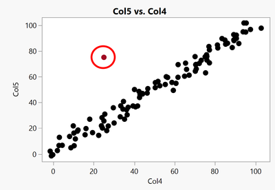
However, if we broaden our scope to two dimensions, we may encounter outliers.


The preceding scenario isn't too dire since we can identify outliers through graphical analysis.
However, what if we're dealing with a plethora of variables, say, exceeding 10?
Robust Median Regression using Anscombe data table
To mitigate the impact of outliers, we can employ robust regression techniques like median regression.
Robust median regression is a statistical method that uses median regression to minimize absolute deviations and is resistant to violations of homoscedastic and normal assumptions.
In JMP Pro, effortlessly apply median regression by selecting the "Generalized Regression" personality and opting for the "Quantile Regression" distribution, specifying the quantile as 0.5 through the Fit Model platform.
The following presents the outcome of median regression applied to the sample dataset "Anscombe" within JMP.


If you are using JMP 18, not JMP Pro 18, you can apply median regression by JMP 18's new feature, Python integration.
import jmp
import jmputils

# Checking installed packages
# jmputils.jpip('list')

dt = jmp.open(jmp.SAMPLE_DATA + "anscombe.jmp")

""""
print(dt.name)
print(f'Number of columns: {dt.ncols}')
dt['y3']
"""

# Install Packages
""""
jmp.run_jsl('''
Python Install Packages("statsmodels")
''')

jmp.run_jsl('''
Python Install Packages("matplotlib")
''')
"""

# Import Modules

import pandas as pd
import statsmodels.api as sm
import matplotlib.pyplot as plt
import numpy as np
from sklearn.linear_model import LinearRegression

# Reshape Data
x = np.reshape(dt['x3'],(-1,1))
y = np.reshape(dt['y3'],(-1,1))
print(x)
print(y)


# Mean Regression vs Median Regression

lr = LinearRegression()
lr.fit(x, y)
beta_ls = lr.intercept_, lr.coef_[0]

q = 0.5
rm = sm.QuantReg(y, sm.add_constant(x)).fit(q, prepend=True)
beta_md = rm.params[0], rm.params[1]

# Print Mean & Median Regression Coefficient

print(beta_ls)
print(beta_md)
The output of beta coefficients are listed LOG windows like below.
(array([3.00245455]), array([0.49972727]))

(4.009997266957748, 0.34500026527269356)
Just to let you know, the following results indicate the mean regression coefficient calculated using JMP.
You can compare the beta coefficients above for both mean and median regression.

Concluding Thoughts;
The demonstration provided offers a foundational understanding of JMP & Python interaction in JMP 18.
Harnessing the power of Python integration within JMP presents an exciting opportunity to elevate your analytical prowess, enabling you to broaden your expertise and achieve more robust insights.