- New to JMP? Let the Data Analysis Director guide you through selecting an analysis task, an analysis goal, and a data type. Available now in the JMP Marketplace!
- See how to install JMP Marketplace extensions to customize and enhance JMP.
Stan Koprowski's Blog
- JMP User Community
- :
- Blogs
- :
- Stan Koprowski
- :
- Single Sampling by Attributes
- Subscribe to RSS Feed
- Mark as New
- Mark as Read
- Bookmark
- Subscribe
- Printer Friendly Page
- Report Inappropriate Content
Single attributes sampling plans or MIL-STD-105E are used when the inspections can only be classified as two outcomes. One can think of this type of plan as go / no-go or in specification versus out of specification. Widely used because all one needs to do is count the number of defects found in the sample or by evaluating the proportion defectives in a process. If large lots are used then the binomial distribution is used. Whereas, the hypergeometric distribution is used when the defects arise from a single lot. When plotting the probability of acceptance against the proportion defective in the lot inspected two curves are possible, Type A and Type B. With Type A, the curve represents the probability that a lot will be accepted against the proportion defective in the lot, where as, with Type B, the curve plots the proportion of lots that will be accepted versus the proportion defective in the producer's process.
The process is to take a random sample of size n from a lot of size N. If the sample is intended to be the lot itself it is considered Type A sampling or Type B sampling when the process is used to produce the lot.
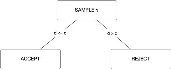
I will show how to generate a single sampling plan by attributes using the two point approach. With the two point sampling plan approach one uses ( p1, α ) and ( p2, β ) for the points. Where by, p1 is known as the Acceptable Quality Limit or AQL, p2 is the Rejectable Quality Limit or RQL, α is the producer's risk and β is the consumer's risk. With the JMP sampling plan add-in one can use either a binomial distribution (Type B) or a hypergeometric distribution ( Type A).
Launch the add-in by selecting JMP Sampling Plans from the Add-Ins menu. Select Attributes-->Single.

You are now presented with three (3) options for lot acceptance sampling plans.
- Evaluate Attributes Plan
- Generate or Create Attributes Plan
- Compare Attributes Plans
I will use the option to generate an attributes sampling plan using the two point method.
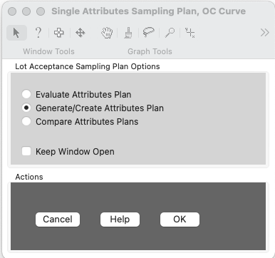
Clicking ok will bring up a dialog to enter the AQL, RQL, α and β, as well as, selecting an option for Type A or Type B analyses when specifying a lot size. Units of Measure will allow one to change the options for p from Proportion Defective, Percent Defective or Defectives Per Million via a drop down menu. When specifying a plan, the primary consideration is the protections provided to both the producer and the consumer.
Enter the following values into the dialog:
AQL = 0.018
RQL = 0.18
Probability of Accepting Lot at AQL (1- α ) = 0.95
Probability of Accepting Lot at RQL ( β ) = 0.10
Notice the Lot Size is optional. If no Lot Size is specified performance graphs will not be displayed.

The JMP Sampling Plan report is produced with details regarding the plan that was created. Let's walk through each outline box to review the contents of the output.
Expanding the first outline node displays the parameters specified to generate the plan.
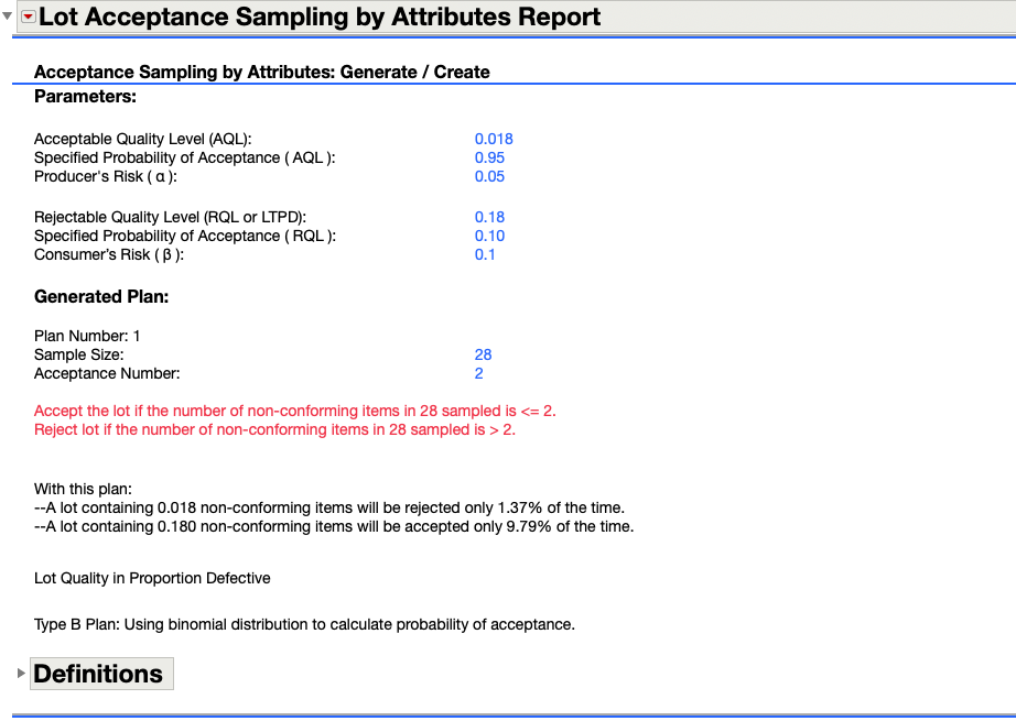
Additionally, the plan created is sample size (n) = 28 and acceptance number ( c ) of 2. If the number of defectives or non-conforming items in the 28 sample is <=2 you would accept the lot. One would reject the lot if the number of non-conforming items is > 2. With this plan and a lot containing 1.8% non-conforming items would only be rejected 1.37% of the time, where as, a lot containing 18% non-conforming items will be accepted 9.795 of the time.
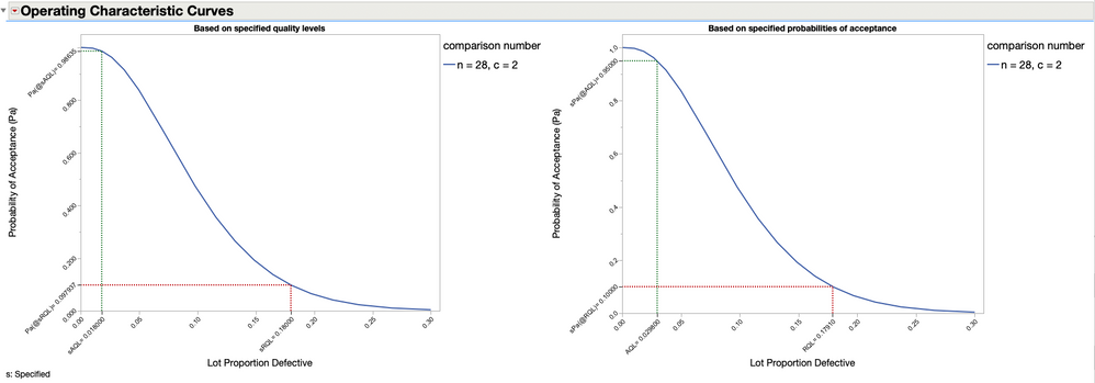
Viewing output from the second outline node displays the Operating Characteristic Curves ( OC ). The OC curves are used to evaluate the insurance offered to both the consumer and producer by the plan. Two OC curves are displayed. The curve on the left is shown using the specified quality levels ( AQL = 0.018 and RQL =0.18) and the associated (calculated) probabilities of acceptance. Where as, the OC curve on the right is shown using the specified probabilities of acceptance ( Pa@AQL = 0.95 and Pa@RQL = 0.1 ) and the calculated quality levels.
Expanding or viewing the last outline node shows a tabular summary of the created plan. The output is displayed showing the desired quality.
The table is color coded to indicate an increase or decrease in associated probabilities of acceptance at both the specified AQL and RQL levels. Better performance than requested for the probability of acceptance at the AQL ( 0.98635 > 0.95) with the blue font and the upward arrow or 0.097937 < 0.1 and the downward arrow at the RQL and same blue font provide quick visuals of the calculated probabilities of acceptance and whether or not they are better or worse from those requested. Similarly, the Associated Quality Level for each specified probability of acceptance is shown. An increase in Associated Quality Level at the AQL (0.029800 > 0.018000 ) denoted by the upward arrow and red font color indicates worse quality than specified. Looking at the Associated Quality Level at the RQL ( 0.17910 < 0.18000 ) shows better than expected results as noted with the downward arrow and blue font.

Now, lets re-run the analysis but this time we will provide a lot size of 10,000. From the red-triangle menu option under the Operating Characteristic Curves select Relaunch Analysis. This will bring up the analysis with the options populated with our previous entries as our starting point. Change the selection from Continuous Sampling Type B (binomial) to Lot Sampling--Type A (hypergeometric) and click OK to continue.
Notice under the Plan Summary outline box of the report additional Performance Measures have been calculated and summarized in tabular format. The output is slightly different from what was presented earlier as we have incorporated a lot size into our calculations and we are now using the hypergeometric distribution. Whereas, previously we used a binomial distribution. Performance measures for Pm, the Average Sample Number (ASN), Average Sample Number (fully curtailed), Average Outgoing Quality (AOQ), Average Outgoing Quality Limit (AOQL), Average Total Inspection (ATI), Average Total Inspection at AQOL, and Actual Risk at Specified Quality for both AQL and RQL are provided.
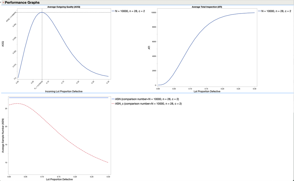
Expanding the outline node for Performance Graphs shows plots for AOQ and ATI. Clicking the red-triangle menu option under the outline node will allow one additional graphs to be displayed including ASN. The ASN curve is displayed with no-curtailment and full-curtailment. Other options include displaying all curves in a single plot or a prediction profiler.
The Average Outgoing Quality (AOQ ) plot shows the AOQ plotted against possible values of proportion defective. The AOQ at the curves maximum is designated as AOQL.
And the point at which the proportion defective occurs is labeled Pm. The AOQ curve is useful when evaluating the effect on average quality going to the consumer after 100% inspection of rejected lots to assess the level of confidence afforded to the consumer after rectification has been completed.
I leave the reader the option to explore the other red-triangle menu options available under the other outline nodes for saving the output or for creating a JMP data table of the plan summary output.
Next time we will take a look at creating Zero Attribute Lot Acceptance Sampling plans, a.k.a., Squeglia plans.
JMP Acceptance Sampling Plan Add-In
Leave me a comment below.
References
Department Of Defense, 1989, Sampling Procedures and Tables For Inspection by Attributes, MIL-STD-105E, https://archive.org/details/MIL-STD-105E_1/mode/2up, Retrieved, April 2021
Schilling, E. G., & Neubauer, D. V., 2017, Acceptance Sampling in Quality Control, 3rd ed., Boca Raton, FL, CRC Press
Montgomery, D.C., 2013, Introduction to Statistical Quality Control, 7th ed., USA, John Wiley & Sons
Grant, E. L., & Leavenworth, R.S., Statistical Quality Control, 5th ed., 1980, McGraw-Hill Book Co.
SAS/QC® 15.2 User's Guide, 2020, Cary, NC
You must be a registered user to add a comment. If you've already registered, sign in. Otherwise, register and sign in.
- © 2026 JMP Statistical Discovery LLC. All Rights Reserved.
- Terms of Use
- Privacy Statement
- Contact Us

