You learned about CUSUM control charts in my colleague @AnnieDudley’s post “How to detect small shifts in Control Charts.” We saw that the CUSUM control chart was better at detecting small shifts than the IMR (Individual and Moving Range) chart. How much better is the CUSUM chart than the IMR chart at detecting small shifts? What is considered a small shift? In other words, how does the CUSUM chart perform compared to the IMR chart?
If this were a hypothesis test, we could measure the α (Type I) and β (Type II) error. This method can’t be used for control charts because control charts are a series of sample by sample hypothesis tests. Instead of the traditional α and β error that is used for hypothesis tests, the Average Run Length (ARL) is typically used to measure the performance of control charts.
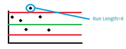 Run Length is the number of samples (subgroups) taken before there is a signal (point beyond the control limits). In the image on the left, the run length is four because there were four samples taken before a point went beyond the upper control limit. Run length is a random variable that can only take on integer values. We need to use the expected value or Average Run Length to measure performance. ARL (Average Run Length) is the expected value of the run length, i.e., the expected number of subgroups until a control chart first signals.
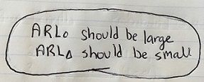 You will hear about two types of ARL discussed in literature: in-control ARL (ARL0) and out-of-control ARL (ARLΔ). ARL0 is the expected number of samples until a control chart signals, given that the process is in control. You can also think of this as sending a false alarm. Since the process is in control (on target), you want ARL0 to be as large as possible. ARLΔ is the expected number of samples until a control chart signals, given the process is out of control (the mean has shifted). You would like for ARLΔ to be as small as possible. If the process has shifted to an unsatisfactory level, you want to learn about it sooner rather than later.
How do you calculate ARL?
 Let’s consider the example used in Annie’s blog post. This example examined data from a car engine thermostat. The engine was designed to operate in a temperature range of [90° C, 110° C]. First let's look at the IMR chart that was used in her post, using only Test 1. We are only considering Test 1 because the addition of run rules makes the determination of a false alarm probability more difficult. With run rules, the probability of a false alarm at a given observation is dependent on the values of the previous observation. This means that the value of α is not constant.
In-Control ARL (ARL0)
α=Pr[Shewhart control chart signals for a given sample | the process is in-control]
1-α=Pr[Shewhart control chart does not signal for a given sample | the process is in-control]
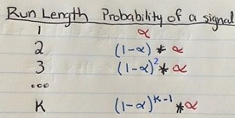
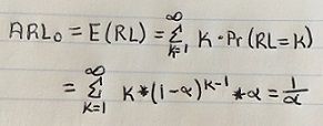
For any Shewhart chart with the usual 3-sigma limits, α=0.0027 is the probability that a single point falls outside the control limits when the process is in control. Therefore, the ARL0 is 1/0.0027≈370. If the process is in control, a signal will be given every 370 samples, on the average.
Out-of-Control ARL (ARLΔ)
1-β=Pr[Shewhart control chart signals for a particular sample | the process is out-of-control]
β =Pr[Shewhart control chart does not signal for a particular sample | the process is out-of-control]
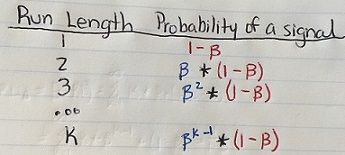
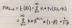
β=φ(zα/2-k)- φ(-zα/2-k)
With 3-sigma limits, zα/2=0.0027/2=3
k=|µ1- µ0|/σ0=|110-103.9632|/ 9.730≈.60204
β=φ(3-.60204)- φ(-3-.60204)=0.9916
ARLΔ=1/(1- β)=1/(1-.9916) ≈119
Although ARL0 is large as we desired, ARLΔ is also large, which we did not want. On average, it would take 119 samples to signal when the mean has shifted from 104 to 110.
CUSUM ARLs
Unfortunately, the ARL calculations for CUSUM charts are not as straightforward. The plotted points are cumulative deviations and are therefore not independent. You can find tables of ARL calculations in textbooks. Lucky for us, JMP can perform these calculations for you. Click on the red triangle next to CUSUM Control Chart – Y and choose “Show ARL.”
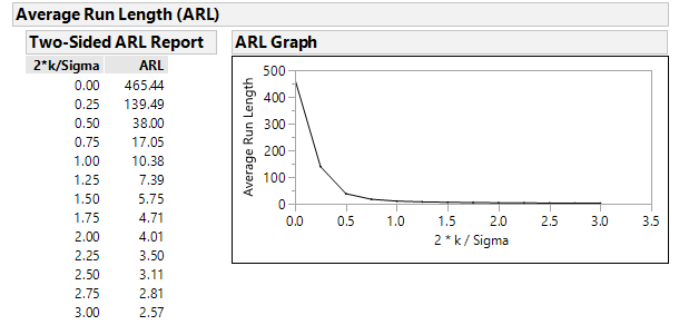
Let's take a look at the in-control ARL: ARL0=465.44, which is good (even higher than the IMR chart). If the process is in control, we expect to get a signal every 465 samples on average. Now let's look at the out-of-control ARL: ARLΔ =10.38. This number is low, which is good (much lower than the ARLΔ for the IMR chart). If the process mean has shifted by 10° C, expect to get a signal every 10 samples on average.
The table below illustrates the ARL performance of a Shewhart control chart and the CUSUM chart with k=0.5 and h=5 (JMP’s defaults).
|
Shift, in multiples of σ
|
Shewhart ARL
|
CUSUM ARL
|
|
0
|
370
|
465
|
|
0.25
|
281
|
139
|
|
0.5
|
155
|
38
|
|
0.75
|
81.83
|
17
|
|
1
|
43.96
|
10.4
|
|
1.5
|
15.97
|
5.75
|
|
2
|
6.3
|
4.01
|
|
2.5
|
3.24
|
3.11
|
|
3
|
2
|
2.57
|
|
4
|
1.19
|
2.01
|
|
5
|
1.02
|
1.69
|
You can see that, the CUSUM chart will detect a shift sooner than Shewhart charts when the shift is less than 2.5*σ. For shifts larger than 2.5*σ, a Shewhart chart will detect the shift sooner.
How h and k affect the ARL
JMP also provides a nifty ARL Profiler. You can find this option under the red triangle beside CUSUM Control Chart – Y.
ARL Profiler, Two-Sided
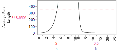
This graph tells us that when h=5 and k=0.5, then ARL2*k/σ=ARL2*0.5/10=ARL.1=348.6502. As you move the slider for h around, you see that decreasing h decreases the ARL and increasing h increases the ARL. Conversely, if you move the slider for k around, you find that decreasing k increases the ARL and increasing k decreases the ARL. You can play with these h and k sliders to determine how altering these values together affect the ARL.
Conclusion
ARL can be used to view the performance of a particular control chart or to compare the performance of different control charts. If the shift is small (less than 2.5*σ), a CUSUM chart will detect the shift before a Shewhart control chart. If the shift is larger (more than 2.5*σ), a Shewhart chart will detect the shift sooner than a CUSUM chart.