What if the nonlinear model you want is not in the Fit Curve platform or the Model Library of the Nonlinear platform?
You can create a model formula in a data table column. If the model is one that you expect to use often, you might consider adding it to the Model Library. (Information on doing so is contained in the JMP Predictive and Specialized Modeling book in the chapter on Nonlinear Regression. Look for the section titled "Customize the Nonlinear Model Library.")
If you recall the calcium example from part 3 in this series, Howard Grimes of Idaho State University did an experiment to determine the amount of radioactive calcium in cells. In particular, the relationship between the amount of time the cells were in a suspension and the amount of radioactive calcium in the cells was of interest. We used the Weibull growth model in the Model Library. However, suppose you are interested in fitting the model in a different form:

This form of the model might be particularly useful as the parameters have a useful interpretation:
𝛽1 the upper horizontal asymptote
𝛽2 the y-intercept
𝛽3 the rate parameter
𝛽4 the shape parameter. If the shape parameter is greater than one the curve is sigmoidal.
To enter this as a column formula in JMP, the first step is to define the parameters and their starting values. To begin, create a new column in the data table and add a column formula. In the Formula editor, change the list choice in the center bottom panel from Constants to Parameters.
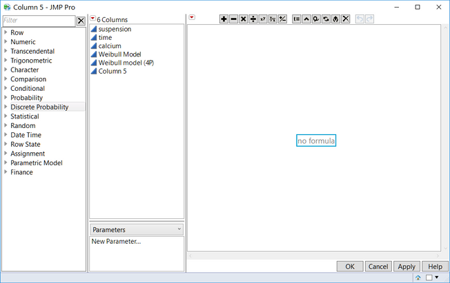
Click on New Parameter. In the dialog box that opens, provide the name of the parameter and the starting value as shown.
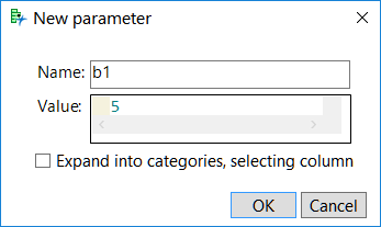
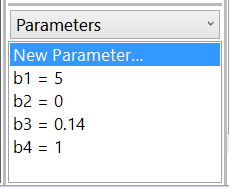
Repeat the process to enter each parameter in the model along with its starting value.
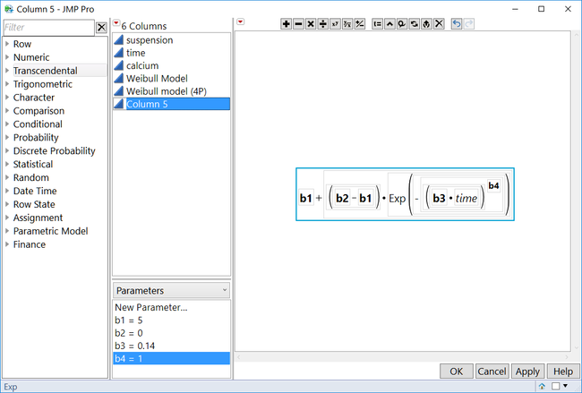
Once you have defined the parameters, you can enter the model formula using the Formula Editior. Note that the parameters will appear as bold entries in the formula.
After the model formula is in the data table with the appropriate parameter starting values, proceed to the Nonlinear platform, entering the Y variable and the model formula column created above as the X, Predictor Formula. After the first set of iterations, this model should have converged. Click on the Confidence Limits button to see the limits around the parameter estimates.
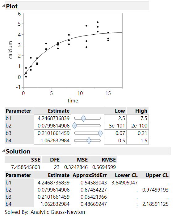
Several of the confidence limits are reported as missing values. The intervals are profile likelihood confidence intervals, and it is not uncommon that the iterative technique used to obtain these limits fails to successfully converge on limits for the parameter estimates.
In examining these results, note that the estimate for parameter b4 is very close to 1. Given that b4 represents an exponent in the model, if it is equal to 1, it has no effect on the computation and does not need to be included in the model. To explore the effect on the model if you fix b4 at 1 first, remember the current solution by clicking on the red triangle and selecting Remember Solution. Name this model Original. This adds a new section to the results window with fit statistics and parameter estimates for the remembered model. Scroll to the control panel in the results window. Change the value of b4 to 1 and click in the square to lock that value. Rerun the model by clicking Go.
Use the red triangle option to remember this solution, and then examine the Remembered Models panel.
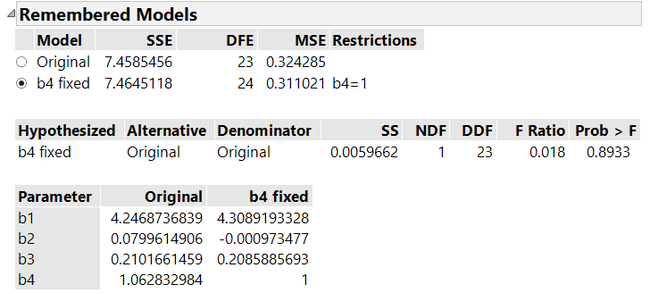
Summary of fit information, the parameter estimates for the new model, and a comparison between the models have been made. In this case, with a p-value of 0.8933, there is insufficient evidence to conclude that the Error Sums of Squares (SSE) of the models are different. This could lead you to conclude that the simpler model is a better choice in this case, and you might choose to remove the parameter b4 from the model equation.
Summing it up
In this series, you have seen three different ways to approach fitting a nonlinear model in JMP: the Fit Curve platform, the Model Library in the Nonlinear platform, and a custom model in the Nonlinear platform. The classic nonlinear approach, using a column formula, is more powerful and flexible, while the Fit Curve platform is easier to use. For those new to fitting nonlinear models, using Fit Curve may be a good way to ease into nonlinear modeling. Once you are more comfortable with specifying models, then the full power of the classic approach in JMP can be explored to expand the types of models available.
Editor's note: Check out the whole four-part series.