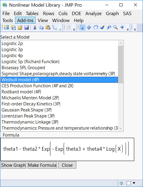
In my previous post, I discussed the use of the Fit Curve platform. Although the Fit Curve platform includes a collection of popular models, it is always possible that you will want to fit a model not available within Fit Curve. The Model Library in the Nonlinear platform provides an alternative way to fit a number of commonly used models. This library provides graphs for many of the models included as well as the capability to use the model graph with the data to set starting values for the parameters. The Model Library is used to create a model formula column for use with the platform.
An example
Let us look at an example of this situation. An experiment was conducted by Howard Grimes, Idaho State University, to determine the amount of radioactive calcium in cells. (His data is used here, with permission.) In particular, the relationship between the amount of time the cells were in a suspension and the amount of radioactive calcium in the cells was of interest. The researchers had reason to believe the response would follow a Weibull growth model. One form of the Weibull growth model is included in the Model Library. To view the Model Library, select Analyze --> Specialized Modeling --> Nonlinear, then click on the Model Library button. A list of the available models is displayed; when a model is selected, the model formula is also displayed. (See JMP Note 60725.)

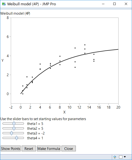
To see the general shape of the model, click on the Show Graph button. Graphs will be shown for most models that have only one X variable. If you are certain this is the model you want to use without looking at a graph, click on Make Formula. You will be prompted to supply the X and Y variables for the model. In this example, select time and calcium for the X and Y variables, respectively. After selecting OK, a graph of the general model form with the points is shown. JMP prompts you to set the starting values for the parameters.
In this particular example, the range used for axes in the graph is much larger than the data. Double-click on each axis to open the axis specification window and change the maximum value and increment for the axis as appropriate. You can then change the parameter estimates by using the slider bar. In this example, previous experiments provide potential starting values: theta1 and theta2 equal to 5, theta3 equal to -2, and theta4 equal to 1. Use the slider or type in these values in the graph window as shown below.

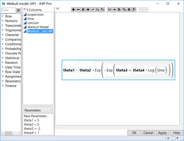
To create a column in the data table with the formula, click Make Formula, then close both the Weibull model window and the Model Library window. Examine the data table to see the column that has been added. You can also view the formula for the column to see both the formula and the starting values for the parameters.

Once the model formula column is created, return to the Nonlinear dialog box and enter the response variable (calcium) and the newly created predictor formula, Weibull model (4P). Select OK. At this point, you have an opportunity to view a plot of the data with the model superimposed and make adjustments to settings as desired. Among the settings that can be changed are the maximum number of iterations, the convergence criterion, and the starting values for the parameters. Click Go to start the iterative process of fitting the model.
The options
Examine the results and pay careful attention to the convergence message toward the top of the control panel. If the model has not converged, you may choose to select Go again to do additional iterations, or you may want to adjust starting values or convergence criteria. Among the numerous options that are available once the model is fit are:
- Save Estimates, which saves the current parameter values to the parameters in the formula column.
- Confidence Limits, which computes confidence intervals around the parameter estimates.
- Remember Solution, which creates a Remembered Models report. Results of remembered models can be compared.
Save Estimates and Confidence Limits are both available as buttons in the results window. Remember Solution is available as an option in the red triangle menu.
Ever the pessimist?
What happens if the model you want to fit is not included in the Fit Curve platform or in the Model Library? That’s a topic for my next installment in this nonlinear modeling series.
You must be a registered user to add a comment. If you've already registered, sign in. Otherwise, register and sign in.