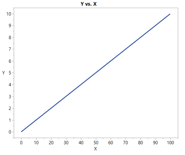
Most of us know what a line is. You can find many definitions, but most of them include the statement that a line is straight; it has no curves. So when we talk about a linear model, we want to go back to that definition of straight. A linear model has no curves, right? WRONG!
A statistician will tell you that a linear model is linear in the parameters. Somehow, that doesn’t seem to help clear things up. So, let’s take a look at some linear models.
A simple linear model in statistics is similar to the line we learned in algebra and can be written:


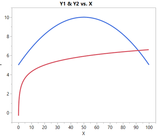
But the models shown in the graph below are also linear models:

These linear models that are not straight lines have formulas like:

In these models, the betas are the parameters and the X’s are the independent variables. So, perhaps the way to look at this is that in a linear model there is only one parameter in each term of the model and each parameter is a multiplicative constant on the independent variable(s) of that term.
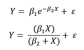
In contrast, a nonlinear model does not have this simple form. Examples of nonlinear models are:

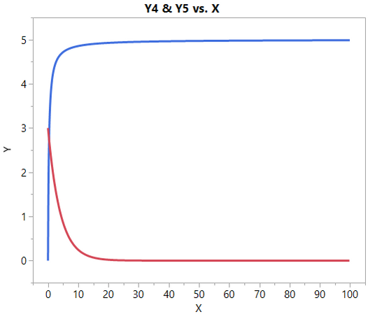
These models may not look very different from the linear models when you graph them:

However, mathematically they are very different because the derivative of these models with respect to any parameter depends on this or other parameters. These nonlinear models require an iterative estimation process, which is much different from using a formula to obtain least squares estimates for a linear model.
Therefore, when fitting a nonlinear model, the analyst must specify the model to be fit, the parameters to be estimated, and the starting values for those parameters. This can be done in JMP using the Fit Curve platform. Alternatively, you can use the Nonlinear platform with a model from the Model Library or with a custom column formula. These options will be discussed in follow-up posts. Look for the next one, which will show how easy nonlinear modeling can be in JMP.
Editor's note: Check out the whole four-part series.