Joining by datetimes

[#1]

Why would you want to join data sets by datetimes?

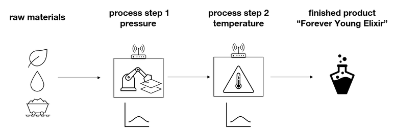
One of the common data preparation challenges scientists and engineers face is matching different data sets by dates, times or datetimes (also referred to as timestamps) (Figure 1).

Figure 1. Example of dates, time and datetime data.

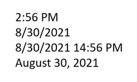
Scientists and engineers often get their metrics from a variety of different measurement systems / pieces of equipment. To analyze their data, they need to combine all the metrics in a single table so that they can look at relationships across all the metrics. 

When you have a unique identifier column or set of columns (e.g. Batch_ID, Lot_ID, UPC, serial number, etc.), joining is relatively simple and can be accomplished using the Tables > Join function in JMP or the virtual join function in JMP. 

It is more challenging when you need to align dates, times or datetimes between data sets. Often the task involves sensors that track metrics continuously over time (for example, temperature, pressure, pH, glucose). To understand how these metrics may impact product endpoints (sometimes referred to as “critical quality attributes”), it will be necessary to create summaries* of those metrics over appropriate time periods. The summaries are then joined with the corresponding product endpoints.

Let’s work through a case study showing how to accomplish this type of joining.

Case Study

Watch the video, or read about the case study below the video.

The process we are trying to understand and improve makes a finished product called “Forever Young Elixir.” The critical quality attribute is Potency. 

A product is being made in two steps. First, the raw materials go into a machine that applies pressure to the raw materials. Then, the assembled raw materials move to a second process step where temperature is applied to create the final product.

Both process steps can be controlled, but today there is a fair amount of variation that we believe is impacting the finished product’s critical quality attribute potency. We are interested in understanding how pressure and temperature impact potency of this product so that, ultimately, we can identify an acceptable operating range for each of the process steps. There are temperature and pressure sensors that monitor the process continuously. 

We will focus on temperature in this example because the process for working with the pressure data is analogous.

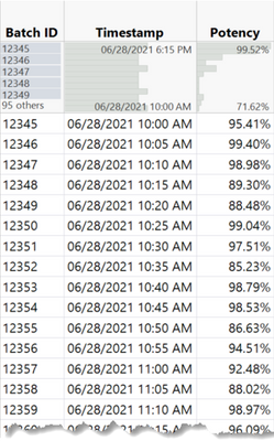
We have a data table that has each lot, the timestamp (datetime) for when the batch was finished and its potency (Figure 2).

Figure 2. Potency data collected for each finished batch along with the timestamp for batch completion.We also have data from a temperature sensor. Temperatures are recorded at one-minute intervals (Figure 3).

Figure 3. Potency data collected for each finished batch along with the timestamp for batch completion.

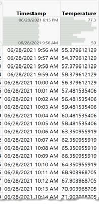
Ultimately, to correlate Potency with Temperature, we need a table with each batch’s Potency and the average* Temperature during the period when the product was made. 

Figure 4. Final analysis table with temperature data combined with potency data. *Other summary statistics could be considered, or one could also explore using the Functional Data Explorer platform which uses all of the data to understand a process instead of summarizing to a single value.

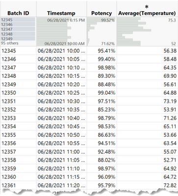
Before we can get into the software, we need to decide which time points in the temperature step are appropriately associated with a particular batch. In other words, when was the batch being processed in the temperature step? 

In discussing with other engineers, we determine that 5 minutes is the length of time a batch is processed in the temperature step. Therefore, the temperature data for the period 5 minutes prior to the batch’s finish timestamp should be used to correlate with the potency of a batch.

Now we have the necessary information to start the data preparation process. 

Note: This example starts with the datetimes already properly coded with correct data type and modeling type. This is a very important step if you want the joins to work correctly. Please jump to the appendix for this blog post if you need a refresher on using dates, times and datetimes.

Video Demonstration

Join in on the joining! Download the two data sets attached below and follow along. If you don’t have JMP already, you can download a 30-day trial.

Review of Steps

1. Decide what range of sensor data readings is relevant to the product.
   • How does my process impact the end point metrics?
   • For each process, what is the time range of sensor readings that is relevant to the final product? 
   • For each process, what is the time range of sensor readings that I want to correlate to the final product?
2. Create a column in the data set with the end point metric(s) that defines the first timestamp for each record that is relevant. 
   • Do this by using a formula column using the finished product’s timestamp (or other reference timestamps if that is not available).
   • You may need to define the last relevant timestamp as well.
3. Join the table with the end point metric(s) to the sensor data using Tables > JMP Query Builder.
   • The join criteria need to be edited to include two conditions: one comparing the sensor timestamp to the finished product table’s timestamp, and one comparing the sensor timestamp to the first timestamp calculated in the second step.
4. Summarize (that is, average) the sensor metric in the joined table using Tables > Summary.
   • Select the sensor metric(s) and then the Statistic desired.
   • Group by all the other columns.
5. Use Graph Builder or Fit Y by X to look at the relationship between Potency and Average Temperature. 
   • Where is potency the highest? 
   • What can this tell you about where to set the operating range for temperature?
   • Consider using modeling techniques so that you can incorporate all of the other process inputs as well.

Please comment on this blog post and let me know if you followed along. I want to know if you found the instructions clear and if not – what I can clarify.  Also, what situations do you have that are not being addressed here?

Appendix

Review of Dates, Times and Datetimes

Let’s do a quick review of this type of data because it is important to get the data type and modeling type correct in all the data tables if you want the data to be joined correctly. Analytic software stores dates, times and datetimes in seconds from a reference date. JMP stores dates, times and datetimes as the number of seconds from 1/1/1904. There is another great blog post on Using Dates, Times, Datetimes and Durations if you want to go deeper on this topic.

If you want to use this type of data (to graph, subtract dates, join via dates), you need to make sure the dates/times/datetimes are formatted as Data Type = Numeric and Modeling Type = Continuous. When you import the data, make sure you do so. For special types of date time formats, you may need to apply a custom import format to let JMP know that it is a datetime. 

Once you format the data as Numeric and Continuous, you will see that the data is represented in seconds. It may look strange to you, but it is correct.

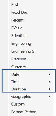
Applying a format is what makes the data look understandable to yourself and others. You can choose from Date, Time, and Duration formats in Column Info (right click on column header > Column Info > Format). Datetimes (timestamps) are in the Time menu (Figure 5).

Figure 5. Format options for Dates, Times and Durations for a column.

Aside

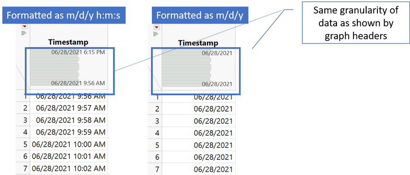
If you want to join two data tables together via datetimes, make sure you have the level of detail necessary to do so in the datetime columns in both tables. The level of detail is determined by the source data. The format does not change the granularity of the data as it is recognized by JMP; it simply changes the granularity visible to us in the cell. 

Let’s consider two scenarios:

1. If your data only has granularity at the date level (no time), applying a timestamp format (e.g. m/d/y h:m:s) will show the m/d/y and then 12:00:00 AM for the time for all records. There is no time detail in your source values, so you cannot compare times within the same day.
2. If your data has detail at the datetime level, applying a Date format (e.g. just m/d/y) will show m/d/y in each cell; however, the underlying granularity will remain (Figure 4).

Figure 6. Timestamp columns with different formats but the same granularity.

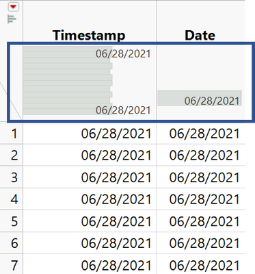
Contrast the two columns (Timestamp and Date) in Figure 7. The same format is applied to both. However, Timestamp has granularity that Date does not, and you can see that in the header graphs in the data table.

Figure 7. Timestamp and Date have the same format but different levels of granularity.

Potency Data.jmp

Temperature Sensor Data.jmp