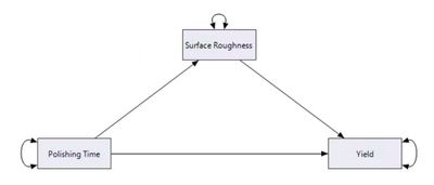
 Welcome to my first post about structural equation modelling and its corresponding platform in JMP Pro. I plan on making this a monthly series with posts explaining the principles of structural equation modelling, as well as how to implement these principles within JMP Pro. For this first post, I will introduce structural equation modelling and then briefly explain where it has been used in the past, as well as where it could be used in the future.
What is SEM?
Structural equation modelling (SEM) is a long-established method for multivariate systems modelling that has seen significant adoption in the behavioral and social sciences. The reason for its popularity in these fields is largely due to its simple visual representation of complex multivariate systems. SEMs are ideal for understanding complex relationships between variables, allowing these complex relationships to be explained to those who have little experience in the field of modelling or in systems of equations. Not only this, but SEM allows the indirect effect of variables to be determined quantitatively, as well as allowing any variable to be modelled as both an input and an output. As a result, SEM can pick up on relationships that may otherwise be missed or confounded when using traditional modelling methods.
Motivation
As a recent chemical engineering graduate, I have taken note of these unique properties in SEM and am interested in exploring its applications in the realm of science and engineering, which is a premise that has yet to be examined. Consequently, I have begun to learn about SEM and how to build, assess and modify these models within the recently added JMP SEM platform. This platform was added in JMP Pro 15 and was the subject of many blog posts. With the arrival of JMP Pro 16, and therefore the addition of many new features within the SEM module, it seemed like a good time to compile a tutorial series to cover my journey into learning about SEM and applying SEM using JMP Pro 16.

I plan to update this running JMPer Cable series as I learn more about the subject and the module as it is developed; this series will also serve as a “getting started” tutorial series for the JMP Pro 16 SEM module. Within this series, I hope to point out common stumbling blocks and address difficult topics that I have tackled recently. Throughout this series, I will show various SEM concepts using short video demonstrations by applying easy-to-understand data sets.
When can SEM be used?
You may wonder why SEM has seen little adoption in engineering while being employed heavily in behavioral and social sciences. There are two main reasons. Firstly, there is a significant barrier to entry to employing SEM in any context since a significant understanding of different statistical metrics and methods is required. Previous SEM software has typically been rather difficult to understand and did not have many comprehensive tutorials associated with them. The JMP SEM platform overcomes the drawbacks associated with other SEM software packages by having an integrated visual analysis platform alongside the statistical outputs, allowing for easy comparison between models.
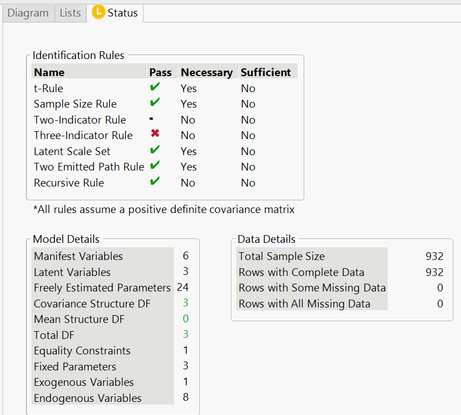
Additionally, users of SEM are required to have deep knowledge of various rules to successfully identify the model and prevent errors in determining a solution. JMP comes with a status window that automatically flags any errors or rule violations that could hinder model identification, coupled with a handy explanation of why the error has occurred and how to potentially fix the error. I will cover this error tab in a later post, but just know at this stage that this has saved me countless hours in debugging and has reduced my frustration with models that do not converge.

Secondly, SEM is typically employed in situations where there is a hypothesized structure for the underlying model, resulting in models that have been created based on user knowledge of the system and relationships between the variables. Then the data that have been collected are introduced to either support or disprove the hypothesis described by the model. In engineering, however, model construction usually follows a data-driven approach where the data collected from experiments or systems are studied to then draw hypotheses and conclusions. This is why other data-driven methods, such as machine learning, are more typically employed in engineering and highlights an obvious issue with applying SEM in this field. I propose that there are a couple of ways that SEM can still be applied, but you will need to wait for later posts in this series to find out more.
Typical issues with SEM

One disadvantage of using SEM is that it requires a large sample size for making reasonable and accurate inferences. The typical observational unit in the context of engineering would be the singular system being studied. When applying SEM to engineering situations, many companies would need to share their data on similar systems for the SEM model to be validated, which doesn’t often happen. However, there are some advanced SEM applications that could be employed to circumvent this issue by using time-dependent process data.
SEM methodology
Since the typical process of fitting SEMs can be thought of as a four-stage method, I will follow this method loosely throughout this JMPer Cable series to explain how each of the concepts relate to this typical methodology. The four stages are as follows:

Thanks for reading, and I hope this has captured your interest in the applications of SEM in engineering as well as the powerful capabilities of SEM and the SEM platform in JMP Pro. I look forward to hearing from you in comments.