- JMP User Community
- :
- Blogs
- :
- JMPer Cable
- :
- Genetic Association with JMP Genomics, Part 6: SNP-Trait Association
- Subscribe to RSS Feed
- Mark as New
- Mark as Read
- Bookmark
- Subscribe
- Printer Friendly Page
- Report Inappropriate Content
JMP Genomics has an array of tools to associate genetic variants with traits. One of the most straightforward of these tools is SNP-Trait Association. By performing this analysis, you can quickly identify significant markers for multiple categorical or quantifiable traits. In this example, we explore ~22,000 markers for histiocytic sarcomas (tumors) in a sample of 474 Bernese Mountain Dogs. The phenotypic classification for this data is binary (either affected or unaffected), but note that this guide works for continuous traits as well as multiple traits.
- From the Genomics Starter Select Genetics > GWAS Testing > SNP-Trait Association.
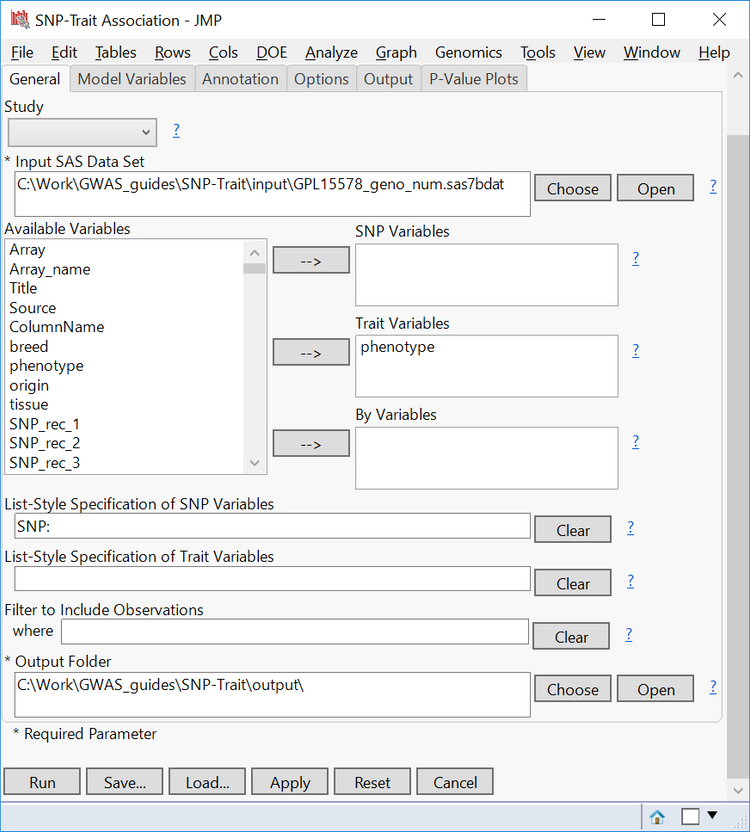
- In the General tab, select GPL15578_geno_num.sas7bdat as the Input SAS Data Set.
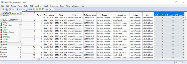
- Note that genotypes have been recoded into numeric format (See Genetic Association with JMP Genomics, Part 1: Importing and Cleaning Data).
- The highlighted columns below begin the marker data.
- In the box labeled List-Style Specification of SNP Variables, type “SNP:” to designate all columns starting with “SNP” as marker columns.
- From the Available Variables box, move phenotype into the Trait Variables Box.
- The By Variables box can be left blank.
- When variables are placed in the By Variables box, a separate analysis will be performed for each unique entry for that variable.
- Specify an Output Folder.
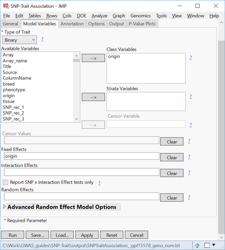
- In the Model Variables tab, select Binary as the Type of Trait. Remember, the phenotypic data for this trait only consists of affected vs. unaffected individuals.
- From the list of Available Variables, select origin and move it to the Class Variables
- Class Variables are variables whose levels form distinct categories in the model. The origin variable, in this case, has distinct levels for the country of origin from which each sample came.
- In the Fixed Effects box, type “origin” to set the variable as a fixed effect.
- Here, you can manually designate Fixed, Random, and Interaction Effects, as well as Advanced Random Effect Model Options.
- Strata Variables are selected to perform a stratified analysis on a binary trait. For this example, leave it blank.
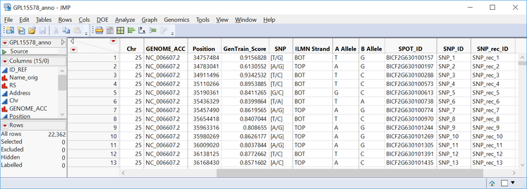
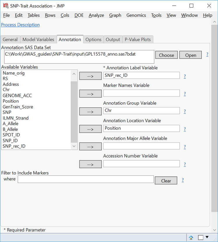
- In the Annotation tab, select GPL15578_anno.sas7bdat as the Annotation SAS Data Set.
- This data set contains annotation information for each marker, like chromosome and position.
- This data set contains annotation information for each marker, like chromosome and position.
- Set SNP_rec_ID as the Annotation Label Variable. Entries in this column will be matched to SNP IDs in the Input SAS Data Set.
- Select Chr as the Annotation Group Variable. This variable will separate the results into different groups, chromosomes in this case.
- Select Position as the Annotation Location Variable.
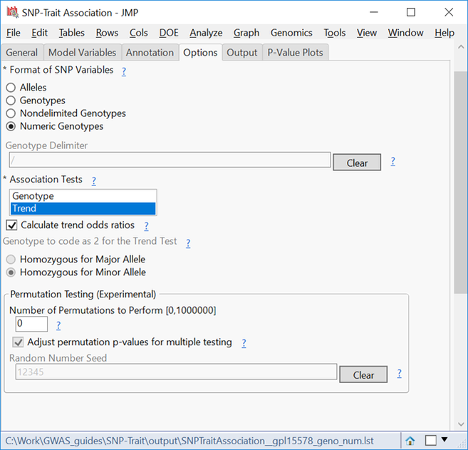
- In the Options tab, select Numeric Genotypes as the Format of SNP Variables
- For these numeric genotypes:
0 = Homozygous for major allele
1 = Heterozygous
2 = Homozygous for minor allele
- Thus, select Homozygous for Minor Allele as the Genotype to code as 2 for the Trend Test
- In the Association Tests box, select Trend. If Genotype is selected, JMP will perform a Pearson chi-square test based on genotypes to determine markers of interest. Since this adds to the computing time, leave it un-selected for this example.
- Check the box next to Calculate trend odds ratios. This is useful for binary or categorical traits.
- The Output tab has options to add analyses to the results. Options include outputting residuals, model fitness statistics, and R-square statistics. Conversely, output can be removed, such as only including markers with significant p-values in the results.
- For the output in this example, leave the default boxes checked. Feel free to experiment with checking boxes and observing the resulting changes.
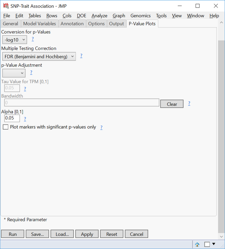
- In the P-Value Plots tab, keep -log10 as the Conversion for P-Values
- For the Multiple Testing Correction option, select FDR.
- When performing multiple tests on the same hypothesis, FDR, or false discovery rate, will reduce the number of false positives.
- If you desire a p-Value Adjustment, one can be selected on this tab. For this example, no adjustment was made.
- Set the Alpha, the level at which a p-value must be for its associated marker to be considered significant, to 0.05.
- Run the analysis.
Results
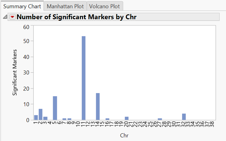
- When the analysis finishes running, the results window will appear showing the Summary Chart This tab shows the number of significant markers on each chromosome.
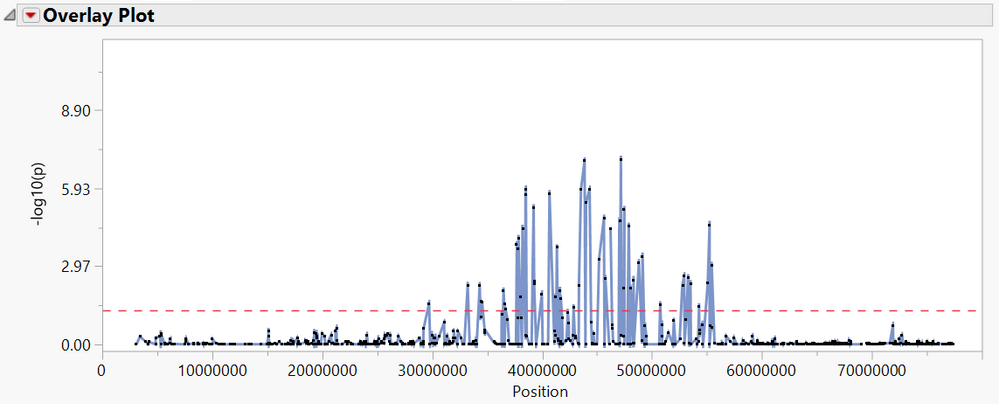
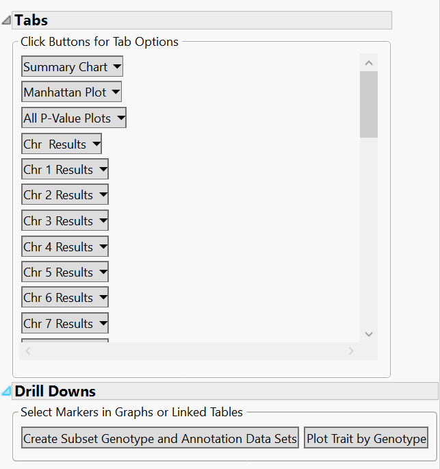
- Each of these chromosomes can be inspected individually by selecting one from the list under the Tabs heading on the left side of the window. Inspect chromosome 11 further by clicking Chr 11 Results. Click View Tab to add the Chr 11 Results tab to the results window.
- Notice the p-values for each marker are plotted by their position on the 11th This information comes from the Annotation Data Set added earlier. Each of the markers that fall above the red dotted line (p = 0.05) are statistically significant.
- Notice the p-values for each marker are plotted by their position on the 11th This information comes from the Annotation Data Set added earlier. Each of the markers that fall above the red dotted line (p = 0.05) are statistically significant.
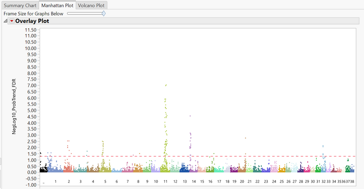
- The Manhattan Plot tab shows a plot of every SNP in the data separated and colored by chromosome number. The y-axis of the Manhattan Plot represents the statistical significance of each marker after the False Discovery Rate correction has been applied.
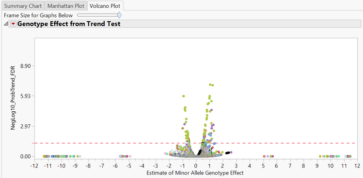
- The last tab is the Volcano Plot Each point on the plot is a single SNP, with the most statistically significant points appearing at the top of the plot. The x-axis shows the fold change for each SNP, with more significant changes appearing at both far sides of the plot.
Drill Downs
On the left side of the results window are Drill Down tools for analyzing markers of interest in further detail.
- First, to create a subset of data, highlight the points on the plots from any of the results tabs, and then click the Create Subset Genotype and Annotation Data Sets button in the Drill Downs
- Note that when points on one plot are highlighted, the same points will automatically be highlighted on the other plots.
- Highlight the two points in the volcano plot with the highest y-value, then click the Create Subset Genotype and Annotation Data Sets A new window will appear with three new data sets. One is the genotypic data from those two markers, one is the annotation data for those two markers, and the last is the other marker data that was not highlighted for the subset.
- Click the Open button next to the Genotype data and the subset will open. Note that this data set only contains two SNPs (SNP_rec_8930 & SNP_rec_15469).
- Click the Open button next to the Annotation data and the annotations for the two SNPs will open. We see that both SNPs are located on chromosome 11.
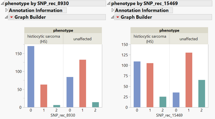
- Return to the results window and click the Plot Trait by Genotype for the two previously selected markers.
- These plots show the distribution of genotypes for both affected and unaffected individuals for each of the markers of interest. The annotation for each of these markers can be viewed by clicking the arrow next to Annotation Information.
- These plots show the distribution of genotypes for both affected and unaffected individuals for each of the markers of interest. The annotation for each of these markers can be viewed by clicking the arrow next to Annotation Information.
*Interactive results from this analysis can be found on JMP Public.
JMP Genomics has many GWAS tools for marker-trait association. The SNP-Trait Association tool is a very quick and easy way to identify markers of interest in large data sets. In this guide, we discovered significant markers for a binary (affected or unaffected) trait. Note that the same tool can be used for all kinds of traits of interest including categorical and quantifiable traits.
You must be a registered user to add a comment. If you've already registered, sign in. Otherwise, register and sign in.
- © 2024 JMP Statistical Discovery LLC. All Rights Reserved.
- Terms of Use
- Privacy Statement
- About JMP
- JMP Software
- JMP User Community
- Contact

