Genetic Association with JMP Genomics, Part 3a: Marker Based Relationship Matrix

[#1]

In JMP Genomics, the Relationship Matrix analysis is used for computing and displaying relatedness among lines. The Relationship Matrix tool estimates the relationships among the lines using marker data, rather than pedigree information (Kinship Matrix tool), and computes the relationship measures directly while also accounting for selection and genetic drift. The Relationship Matrix computes one of three options: Identity-by-Descent, Identity-by-State, or Allele-Sharing-Similarity. Output from this procedure can serve as the K matrix, representing familial relatedness, in a Q-K mixed model. This post will focus on the Relationship Matrix using a data set containing 343 rice lines with 8,336 markers.

Relationship Matrix:

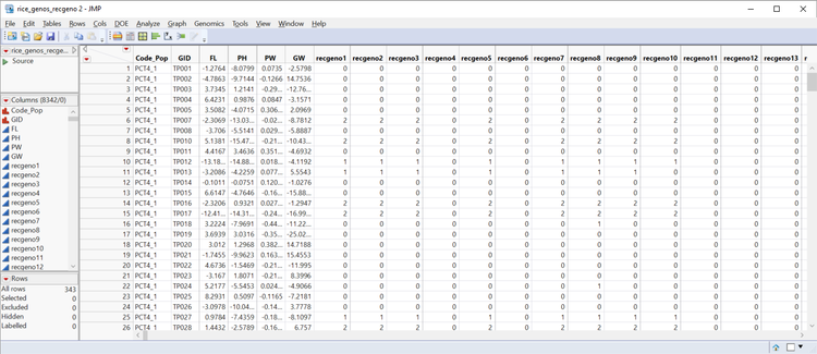
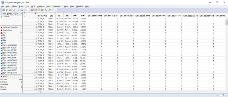
1. Open the rice_genos_recgeno.sas7bdat data set and inspect it in JMP. It has 343 rice lines in rows, six columns of annotation and phenotypic data, and 8,336 columns with marker data. These markers are coded as numeric genotypes. This format is required for the Relationship Matrix. For more information on numeric genotypes and recoding, see the earlier blog post, Genetic Association with JMP Genomics, Part 1: Importing and Cleaning Data.
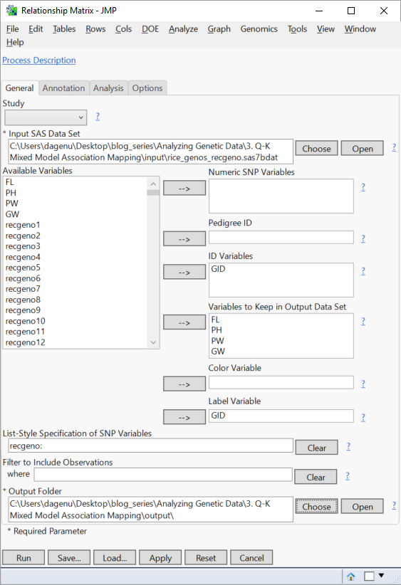
2. From the Genomics Starter menu, choose Genetics > Relatedness Measures > Relationship Matrix.
3. Select rice_genos_recgeno.sas7bdat as the Input SAS Data Set.
4. Select the GID variable from the Available Variables list and place it into the ID Variables and Label Variable
5. Select the phenotypic variables, starting with FL and ending with GW, and place them in the box labeled Variables to Keep in Output Data Set. The traits measured are as follows:
   • FL: days to flowering
   • PH: plant height
   • PW: panicle weight
   • GW: grain yield
6. In the box labeled List-Style Specification of SNP Variables, type “recgeno:” (without the quotes) to select all variables starting with the prefix “recgeno” as marker variables.
7. Choose an Output Folder.
8. In the Annotation tab, select rice_anno_recgeno.sas7bdat as the Annotation SAS Data Set.
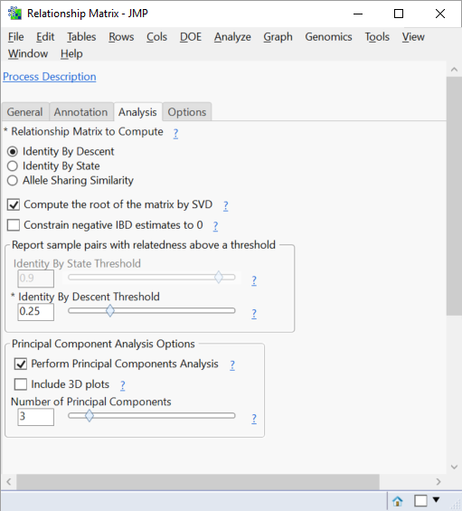
9. In the Analysis tab, leave the Identity By Descent option selected.
   • This will estimate the probability that individuals in the relationship matrix share an allele from a common ancestor at a specific locus. As noted above, options are available for Identity By State and Allele Sharing Similarity which use Gower’s Similarity Metric to estimate the probability of two individuals sharing the same allele regardless of inheritance with and without a Range Standardization, respectively.
10. Check the Compute the Root of the Matrix by SVD
    • This option produces a file containing the square root of the relationship matrix, which will be used later in the QK association analysis.
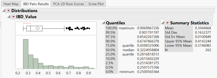
11. The Identity By Descent Threshold slider can be changed to alter the threshold of IDB for pairs to be reported in an output dataset. The default setting is .25, meaning all pairs of rows with an IDB value greater than or equal to .25 will be included in the output dataset rice_genos_recgeno_prs.sas7bdat.
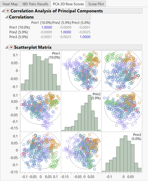
12. In the Principal Component Analysis Options, JMP gives options to perform PCA and set the number of Principal Components to include in the analysis.
    • Principal Component Analysis is a tool to combine input variables in a way that eliminates the facets of variables that do not explain variance in the data. The number of components will designate how many smaller factors will be used as new variables account for as much of the overall variance as possible without bloating or overfitting the model.
13. In the Options tab, check the box labeled Plot Relationship Matrix Heat Map. If you would like to append a prefix to the output variables, it can be done in this tab as well.
14. Click Run to start the analysis. Examine the Heatmap Results in the first tab of the results dashboard:

Results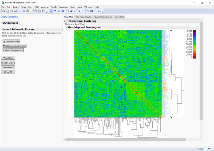

• The Heat Map tab displays the relationships among the 343 lines. The red diagonal represents perfect relationship of each line with itself; the symmetric off-diagonal elements represent relationship measures (in this case IBD) for pairs of lines. The blocks of warmer colors on the diagonal show clusters of closely related lines.
• The dendrogram (tree diagram) on the right shows the results of a cluster analysis on the IBD matrix. Double-click on any branch to zoom in and inspect the members. To revert to the top-level view, click on the Hierarchical Clustering hotspot (red arrow) and choose Release zoom.

15. Return to the results dashboard, and view the IBD Pairs Results
    • The histogram shows the distribution of IBD scores for the 262 pairs of lines with IBD values greater than 0.25. A dataset of these pairs has also been saved to the specified Output Folder titled rice_genos_recgeno_prs.sas7bdat. This table is also viewable by clicking the View Data button under the Launch Follow-Up Processes menu.
16. Look at the PCA 2D Row Scores

• This Scatterplot Matrix shows the correlations between each of the three principal components. There is not evidence for strong population structure in these results because there isn’t any stratification of points in these scatterplots.

17. Examining the Scree Plot tab shows the proportion of the variance accounted for by each Principal Component. In this case, the first two Principal Components account for most of the variation.

K-Matrix Compression (optional)

Q-K association analysis is computationally intensive and the part incorporating the K matrix is especially time-consuming. There is a technique for reducing the number of variables required to represent the familial relatedness between lines. With fewer variables each model, run time is significantly reduced. The technique is called K Matrix Compression. It can be performed in JMP Genomics as part of the Genetics Q-K Analysis Workflow (which you can learn about in a later blog post), or as a free-standing process. The algorithm optimizes the compression for one trait variable at a time, so it needs to be repeated for each trait to be analyzed.

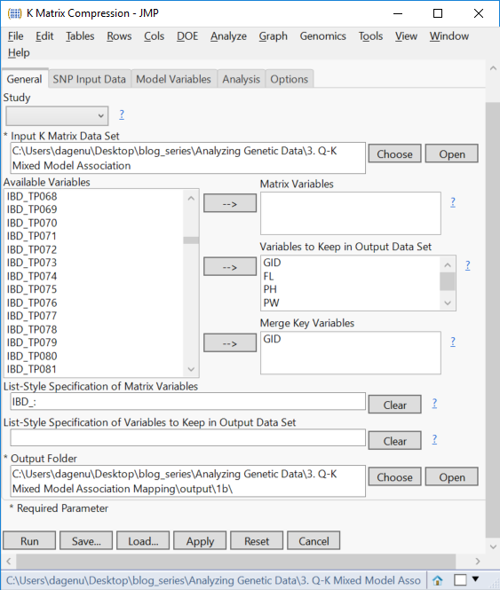
18. From the Launch Follow-Up Processes menu, select K-Matrix Compression. A new dialog box will be launched, with the General tab showing the applied settings from the Relationship Matrix analysis, and a matrix of Identity by Descent values as the Input K Matrix Data Set.
19. Select GID and move it to the Merge Key Variables
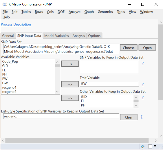
20. The SNP Input Data tab has the SNP Data Set already selected. The Trait Variable will have to be selected manually. Recall that compression can only be performed for one trait at a time. For this example, select GW as the Trait Variable, and designate GID, FL, PH, PW as Other Variables to Keep in Output Data Set.
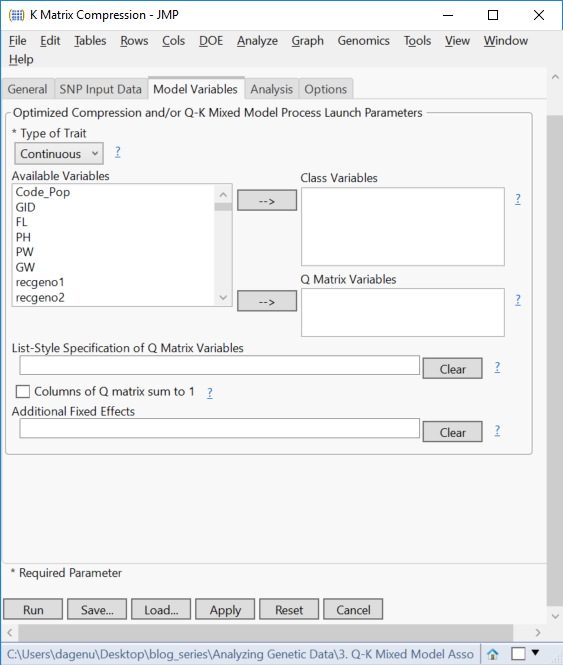
21. On the Model Variables tab, set the Type of Trait to Continuous. There are no Class Variables in this data set nor Q Matrix Variables. The Q Matrix will be assembled in a later post.
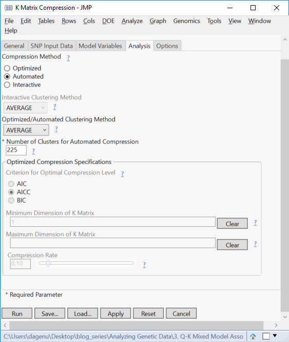
22. On the Analysis tab, set the Compression Method to Automated.
23. Clusters can be constructed using different Automated Clustering Methods. For this example, select AVERAGE from the dropdown menu.
    • This will set the distance between clusters to the average distance between pairs of observations, creating clusters with similar, small variances.
    • For descriptors of each of the possible methods, click the ? icon next to the drop down menu.
24. Select 225 for the Number of Cluster for Automated Compression. This will compress the K matrix, a square matrix, to these dimensions.
25. Click Run to begin the compression. When the process is complete, a SAS output window will appear along with the newly compressed K matrix, rice_genos_recgeno_ibd_kc.sas7bdat.

*The interactive results from this analysis are available on JMP Public.

Summary

This document served as a walkthrough for creating a Relationship Matrix from a data set containing 343 rice lines with 8,336 markers. This relationship matrix was composed of Identity By Descent values, but can be calculated for Identity By State and Allele Sharing Similarity as well. This process estimated the relationships among the lines using marker data since no pedigree information was available. Additionally, this post covered K-Matrix Compression, which can be used to reduce computing time in Q-K Association Analysis while still producing similar results to analysis with an uncompressed matrix. 

rice_genos_anno.zip