This blog discusses how to address constraints problems when using design of experiments (DOE) for a mixture where the mixture components have different variants and different concentration ranges for each variant. This is an expansion of the Discovery Summit presentation by @chris_gotwalt1 about how to approach difficult constraints when working with continuous factors. This blog will go a step further to tackle mixture designs with variant-specific constraints specifically.
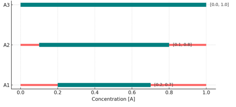
Let’s discuss what we mean by mixture designs with variant-specific constraints. In the example below, we have a mixture of A, B, and C components. Component A, however, can come in three different variants: A1, A2, and A3, with each having its own allowed range of concentration (shown below).

Figure 1: Allowed (green) vs. disallowed (red) ranges of concentration [A] based on variants A1, A2, and A3.
The desired outcome of the DOE is shown in the ternary plot below where using variant A1, [A] in the DOE has a value between [0.2 – 0.7]; for A2, A=[0.1 – 0.8]; for A3, A=[0 – 1].

Figure 2: Desired DOE run locations in ternary mixture space with variable A constraints.
Components B and C might have their own variants also, but for simplicity, let’s focus on component A for now.
One might think we can simply add “Disallowed Combination Filter” on mixture factors the same way we can add them to continuous and categorical factors. When working with mixture designs, however, there is already a constraint on the summation of the mixture factors, and a design convergence issue would occur if additional constraints are added (see below).

Figure 3: DOE interface when attempting to add mixture constraints directly.
How can I add constraints to a mixture design and specify the different ranges for each of the variants of A? Well, let’s see together!
Step 1: Create a candidates data table.
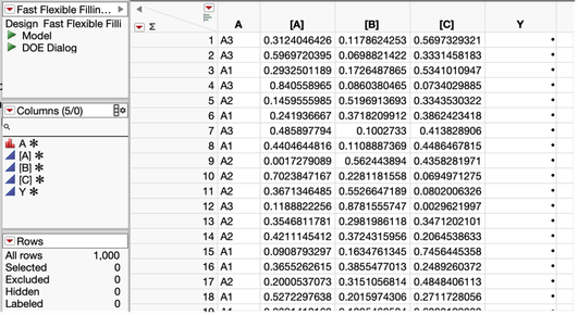
- Create a candidates data table of 1000 possible combinations to ensure the design points spread well across the entire experimental space. This can be achieved using a Space Filling Design by going to DOE -> Special Purpose -> Space Filling Design.
- Add the categorical and mixture factors as shown in the figure below.
- Add a 3-level Categorical factor, call it A, and then add A1, A2, and A3 as its values.
- Add three Mixture factors [A], [B], and [C] with 0 and 1 being their ranges.
- For Number of Runs, choose 1000.
- Select the “Fast Flexible Filling” option. It is the only option that works with the mixture components.
- Click"Make Table" at the bottom.

Figure 4: DOE interface when creating a space filling design for 1000 candidate runs.
The candidates data table would look similar to the following:

Figure 5: Fast flexible filling design output data table used as a candidate set of 1000 potential runs.
Step 2: Remove the undesired ranges for each variant of A.
Remove the undesired ranges for each variant of A using the Multivariate platform and the local data filter to select the unwanted ranges.
- Go to Analyze --> Multivariate Methods --> Multivariate. Select [A], [B], and [C] for the Y, columns.
- Add the local data filter and select the categorical variable A. Click the AND button, and select the concentration of A variable. The goal here is to select the undesired combinations of A= A1 and the range of 0–0.2 and 0.7–1 for the concentration [A]. To do so, I found it easier to type in the desired range (e.g., 0.2–0.7), click the red triangle on the concentration range filter, and click Invert Selection to get the range of 0–0.2 and 0.7–1 selected.
- Select the points in the graph using a regular left-click or using the Lasso tool for a more defined selection. In the video, I used the Lasso tool to select all points.
- Make sure the data points are now selected in the data table as well. Delete the points from the table.
- Repeat the same steps, but this time select A2 for category A AND [A] concentration of 0–0.1 and 0.8–1.
Watch how to do this in the video below.
Video: Using the multivariate report with the local data filter to remove the undesired concentration ranges from the candidate runs tables.
If the variants vs. concentration is plotted, the graph would look like the following one. You can see how this looks similar to the first figure's concentration range of A as a function of its variant.

Figure 6: Scatterplot distribution of the candidate runs after constraints are added.
Step 3: Use the “cleaned” data table as a Candidate Set in the DOE platform
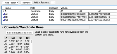
First, go to DOE -> Custom Design. Click "Select Covariate Factors" under Covariate/Candidate Runs.

Figure 7: Outcome when Covariate/Candidate runs column [A], [B], and [C] are added using the Select Covariate Factors button.
Next, follow these steps:
- Create your model by adding the Main Effects and/or the Scheffe Cubic terms.
- Set the Number of runs to 18 matching the number of runs originally recommended without the candidate runs. This is my recommendation, but you might decide to take another approach on how to choose the total number of runs.
- Select "Make design" and "Make Table."
- Add a marker to the rows by going to Rows -> Color or Mark by Column, and choose the A variant column to differentiate the experiments using A1 vs. A2 vs. A3.
- Change the number of decimals in columns [A], [B], and [C] to show only two decimals by going to the Column Properties -> Format -> Fixed Dec -> Dec=2.
- Create a Ternary plot by going to Graph -> Ternary Plot and placing the [A], [B], and [C] factors in the X plotting role. With some annotation and added reference ranges, one can see that the newly designed 18 experiment runs addresses the constraints related to component A variants.

Figure 8: (a) Created DOE table with applied constraints on [A] based on its variants, and (b) the resulting ternary plot showcasing the used ranges of [A] based on its variants A1, A2, and A3.
Step 4: Run the experiments and test the model
- After you run the experiments, fill out the value for the Y response, go to Analyze -> Fit Model, and run the model.
- Add the profiler to the report to visualize the effect of the variants of A and the concentrations of the three components A, B, and C.

Figure 9: Prediction profiler of model created using simulated Y responses.