Welcome back to my series on structural equation modelling (SEM). So far in the series, I have introduced SEM, explored why we might want to employ SEM and discussed the basics of how to set up path diagrams. Just to recap this idea, the reason that SEM is useful is that it allows the modelling of concepts in the form of latent variables. Additionally, SEM allows for variables to be used as both inputs and outputs in a system, which is typically the case for engineering variables. Hopefully, as I build up these concepts, these advantages will become clear.
Path diagrams are a big topic that could be discussed for hours. Therefore, it is my aim to cover the aspects of path diagram construction that I consider to be key when starting out.
In this post, I explain degrees of freedom in SEM, how to construct path diagrams with latent and manifest variables, and some common issues that can occur in path diagram construction.

Degrees of Freedom
I am assuming that since you are reading a blog post about a multivariate modelling technique, you are at least somewhat familiar with the basic concept of degrees of freedom (DF). A short reminder of the topic, in standard statistical modelling, DF is about ensuring that you have at least as many observations as parameters to estimate. This is a requirement for the model to be identifiable, or in other words, for the model parameters to be estimated.
In the context of SEM, DF are calculated by subtracting the number of parameters that need to be estimated from the number of variances and covariances in the system. So, in this context you can see that the way we calculate DF is actually a little different since it relies not only on the number of variables in the system but also on the number of connections between the variables. We must have a DF of at least 0 for the SEM to be identifiable; any less than this and the model parameters cannot be estimated.
I could bore you with the equation of how to calculate DF or spend a page showing you how we derive the equation. But it is far better to just illustrate to you that JMP Pro can do this calculation for you.

As you can see from the image above, when you set up your path diagram, JMP Pro gives you some details regarding DF. In this example, you can see that we have two manifest variables, one latent variable and therefore -1 DF. This means that in this case, unless we can find a way of increasing the degrees of freedom, the model will be unidentifiable, and therefore no solution will be found. The obvious next question is “How do I increase the DF of the system?” This can be tackled in a few different ways traditionally. However, since we have JMP Pro to help us, we are going to take a look into the status tab that it provides to see if it helps us find how to fix our problem (in the video below).
Path Diagrams Extended
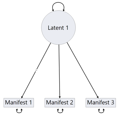
As I mentioned in my previous blog post, we will look at the construction of path diagrams when we have latent variables in our system. Coincidentally, constructing path diagrams with latent variables and the idea of degrees of freedom are linked in SEM since the number of latent variables affects DF. In the video below, I demonstrate both of the concepts outlined above to build a path diagram with real data containing only one latent variable.
Common Issues
Now that you have seen some more features of path diagram construction in JMP Pro, I want to share with you some common issues that I have personally faced when starting path diagram construction, in the hopes that you can avoid the same issues.
The problem I want to focus on here is one that I had when I first started using the solvent data set that I’ve explored in a few of my posts. Hopefully, this issue highlights the importance of always checking the status window. When I first tried to build the path diagram for this data set, I had an amber warning in the status area. Usually, I would ignore an amber error since it is an error that doesn’t need to be fixed for the model to run.

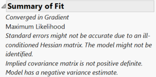
The issue with the data is that the scales of two of my manifest variables are drastically different. This did indeed cause some strange results from the analysis, and when I ran the model without fixing this issue, I was greeted with a string of errors in the Summary of Fit section.

When I first saw this error, I had no idea how to fix it. So I went back to the status window in JMP Pro and discovered the issue was already reported before the analysis took place.
Fortunately, JMP provides the ability to create formula columns where we can just apply the standardization formula to each column. When using data in a path diagram, it is fine to standardize it. This is because in SEM we are only interested in the correlations between variables; the scale is added by the SEM constant (see my Discovery Summit post for more on this). Through standardization, only the scale is lost, so no relevant data is lost in this case. Once the transformation was applied, I just used the new data with the old model, and the model converged nicely. This should highlight the importance of data preprocessing when creating path diagrams.
Thanks for tuning into this month’s installment of SEM. I’d like to encourage my readers to post their common issues and solutions in the comments below. See you next month for more SEM!
You must be a registered user to add a comment. If you've already registered, sign in. Otherwise, register and sign in.