As part of my work with JMP, I have been exploring how structural equation modelling (SEM) can be applied to help solve science and engineering problems. One of the ideas that I have tried is to use SEM for fault detection in large-scale chemical processes. This would work by constructing an SEM on in-control data from a process and then applying this model to out-of-control data to see if it is possible to detect changes to the system.
My aim with this post is to share a small part of this exploratory process to highlight the potential value of applying SEM to problems previously not considered in this way. To do this, I will briefly explain where I got my data from, then I will go through the process from start to finish. This should provide a general tutorial on how to set up a basic SEM in JMP Pro.
Tennessee Eastman Simulator
To perform an analysis of this caliber, I first needed a data set of sufficient size. Chemical process data sets are hard to get access to since companies don’t disclose their exact manufacturing details. Luckily, there is a simulator called the Tennessee Eastman Simulator (TES) that allows data sets to be generated for a large chemical process, along with data after a fault is introduced to the system.
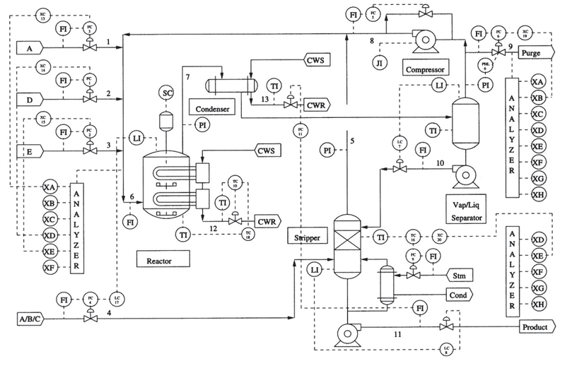
The image above is called a Piping and Instrumentation Diagram (P&ID) and is used to show many things about a system, but in this case, it is used so that we can see where and what measurements are being taken. Don’t worry if the full TES P&ID is confusing. When we start to construct the SEM, the system will reduce in complexity dramatically. But this poses the question: How far can we simplify our model and still obtain meaningful results? I will explore this idea towards the end of the example.
In this case, one of my former colleagues, Jeremy Ash, provided me with a baseline data set from the simulation, along with three other data sets from the system after different faults were introduced. To keep things simple, I decided to just use the baseline data set and the data set from fault 1, which was an error in the A/C feed ratio.
Exploratory Data Analysis
To demonstrate as simple of an example as possible of SEM in an engineering context, I performed various analyses on the data set to try and find a way to reduce it. This is necessary since this data set contains more than 50 variables (that is, without taking time into account, which will be covered in another post), which means the system will rapidly become very complicated. For simplicity's sake, only seven variables were selected to be used in the construction of the SEM; this number was a somewhat arbitrary choice, and you may wish to have more or less variables than this. It all depends on the tradeoff that you are willing to accept between simplification and lost relationships in the data.
In this control case, we know what the fault is that causes the deviation from normal operation: the A/C feed ratio. Therefore, in an effort to keep this SEM simple, I designed the model to detect this one fault only. At this point, you can see how these design choices dramatically affect the quality and usability of the model. In this case, the model created would not be able to be extrapolated to robustly detect other faults that may occur.
Without going into too much detail of my personal exploratory process, I have included the correlation maps for the entire datas et and the reduced data set so that you can see that the variables that have been selected have a very strong correlation with each other. This, of course, is a vitally important part of constructing a SEM. If none of our variables have a significant correlation, then no latent factors can be found, and no SEM can be constructed!
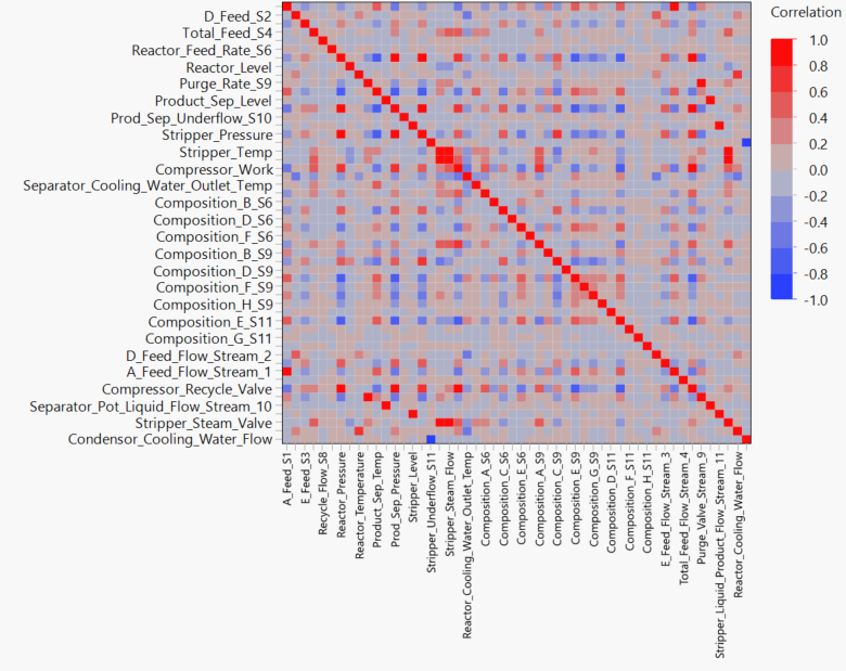
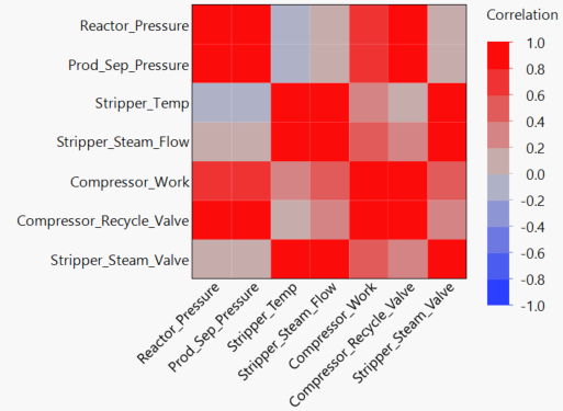
Hopefully, the size of the initial correlation matrix should highlight why I decided to reduce the data set so drastically for this example. I should point out here that in my EDA I found that the “A flow” and “C flow” variables were highly correlated to the other variables, but I didn’t include those in the matrix. This is because we know that the error is due to these variables. Therefore, I studied the correlation matrices before and after the error occurred to monitor this difference. These variables will be considered in the final model though, since they are clearly very important for identifying when and why the error occurred.
Reduced Model
Now that the data set has been simplified, it becomes a lot easier to analyse the data and construct a structural equation model. Therefore, the next step is to perform a factor analysis to determine how many factors should be used in the SEM.

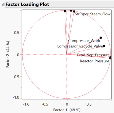
Here you can see that 95% of the data is represented through two factors, while 98.5% of the data is represented through three factors. This means that when we construct our SEM we should use two or three factors. JMP Pro also provides us with the factor loadings, showing us the correlation between each of our manifest variables and latent variables. Therefore, this serves as the basis of the SEM construction. If we compare these factor loadings to the seven-variable correlation matrix, we see that the factor loadings agree with the correlation analysis.
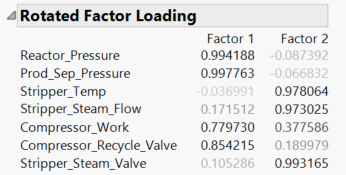
I’d like to point out here that the compressor work and the compressor recycle valve do not have as strong factor loading to the factors as the other variables do to their respective factors. This will be important when it comes to building the SEM, with the conclusion being at this stage that these two variables would be more strongly correlated to the potential third factor.
Identification of Factors
Let’s take a moment to actually understand what all the factor information from the last section is telling us. If we take factor 1 to begin with, we see that two of the associated manifest variables are pressure measurements. While the other two variables are to do with the compressor -- since the compressor's job is to increase the pressure of the system -- these two variables must also be related to the system's pressure. This means that each of our manifest variables here are indicators of latent factor 1, pressure.
Looking at factor 2, a similar relationship can be found. Each of the manifest variables here are related to temperature in some way: the stripper temp, steam flow variables and a slight correlation to compressor work, which would add some energy to the system. Therefore, latent factor 2 must be related to temperature of the system.
Anyone familiar with chemical engineering systems will know that both temperature and pressure are critically important to any industrial process and are both closely related. Again, this is an important relationship to know of regarding what is happening in the real system and so is potentially important when constructing the SEM, too.
Conclusion
By performing exploratory data analysis with JMP Pro prior to constructing the SEM, we have managed to identify key relationships and factors in the system. These preliminary findings give a clear scope for the development and comparison of SEMs.
Next month, I will construct the SEM for the system and use it to try and detect when and where a fault occurs in the system.