- New to JMP? Let the Data Analysis Director guide you through selecting an analysis task, an analysis goal, and a data type. Available now in the JMP Marketplace!
- See how to install JMP Marketplace extensions to customize and enhance JMP.
JMPer Cable
A technical blog for JMP users of all levels, full of how-to's, tips and tricks, and detailed information on JMP features- JMP User Community
- :
- Blogs
- :
- JMPer Cable
- :
- Cross Evaluation and Progeny Simulation with JMP Genomics, Part 2: Predictive Mo...
- Subscribe to RSS Feed
- Mark as New
- Mark as Read
- Bookmark
- Subscribe
- Printer Friendly Page
- Report Inappropriate Content
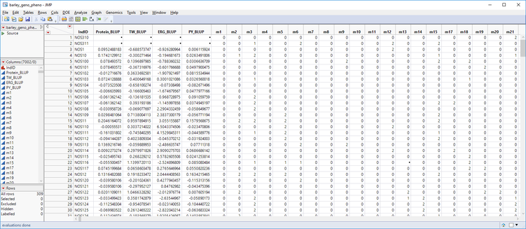
In last week’s post, we consolidated breeding trial data into a single table using Best Linear Unbiased Prediction. The table below (barley_geno_pheno.sas7bdat) shows ~300 barley lines with phenotypic values for four traits and ~7000 genetic markers. In this post, we will use the Predictive Modeling Review tool in JMP Genomics to create multiple models and compare them via cross validation. After cross validation, we will select the most effective model and use it to create scoring code files from which we can perform Cross Evaluation and Progeny Simulation.
Impute Missing Genotypes
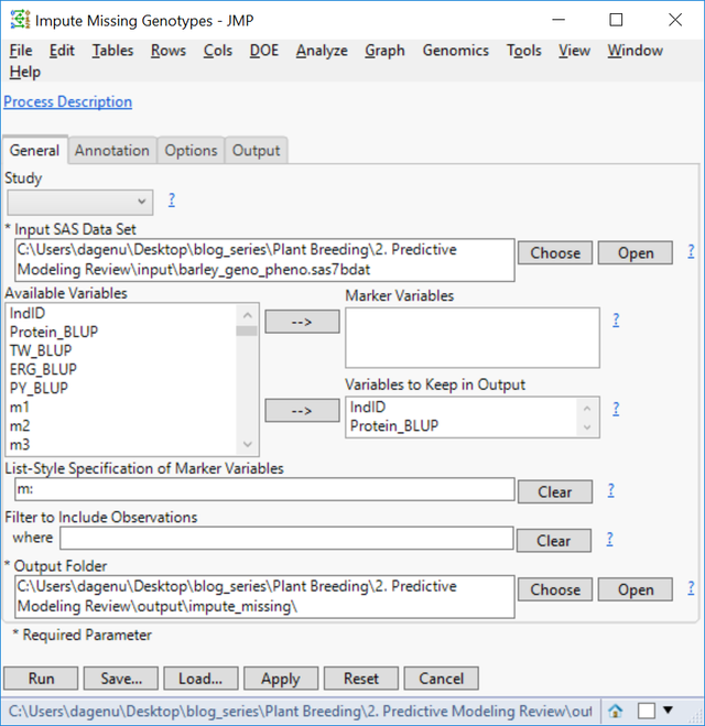
- Note that in the data set shown above, some of the marker data is missing. Before running the Predictive Modeling Review tool, these missing genotypes will need to be imputed. JMP Genomics has a tool to impute missing genotypes based on a nearest neighbor sample. To access this tool select Genetics > Genetics Utilities > Impute Missing Genotypes from the Genomics Starter.
- On the General tab, choose barley_geno_pheno.sas7bdat as the Input SAS Data Set.
- Select IndID, Protein_BLUP, TW_BLUP, ERG_BLUP, and PY_BLUP as Variables to Keep in Output.
- In the List-Style Specification of Predictor Continuous Variables box, enter m: to designate each column beginning with the letter “m” as a marker variable.
- Select an Output Folder.
- There is no annotation data set for this example, so the Annotation tab can be left blank.
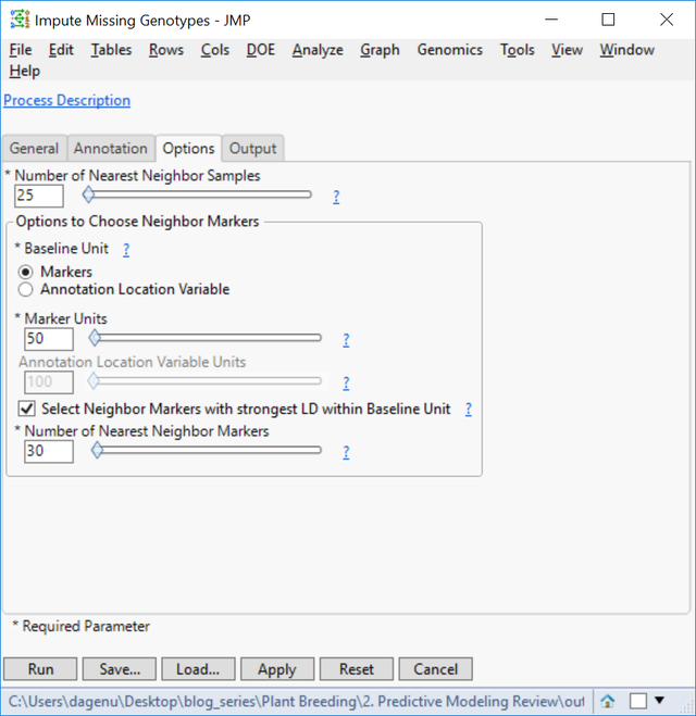
- On the Options tab, set the Number of Nearest Neighbors Samples to 25. This will use a marker’s nearest 25 neighbors to impute the missing genotype.
- In the Output tab, type barley_impute into the Output File Prefix
- Click Run to begin the analysis. When the process finishes, the new dataset will appear in your designated Output Folder. This imputed data set titled barley_impute_img.sas7bdat will be used for the Predictive Modeling Review input below.
Predictive Modeling Review
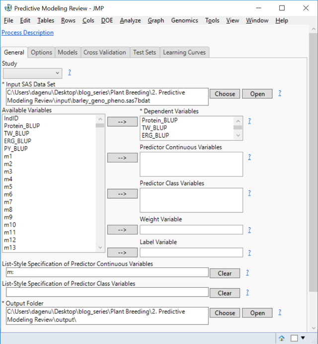
- From the Genomics Starter menu, select Predictive Modeling > Main Methods > Predictive Modeling Review. On the General tab, choose barley_impute_img.sas7bdat as the Input SAS Data Set to populate the Available Variables box.
- Place each of the four traits in the Dependent Variables. JMP will create models for all four traits simultaneously.
- In the List-Style Specification of Predictor Continuous Variables box, enter m:
- Select an Output Folder.
- Leave the default selections on the Options tab.
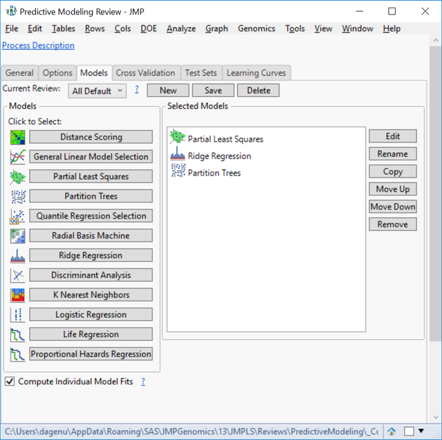
- In the Models tab, there are 12 types of models, which are all fully customizable. For this example, choose Partial Least Squares, Partition Trees, and Ridge Regression. We will create these three models to predict each of the four traits and compare their effectiveness using cross validation.
- Individual model settings can be adjusted by highlighting the Selected Model of choice and clicking Edit on the right of the window.
- Also, multiple iterations of the same modeling type with different settings can be included in the same analysis.
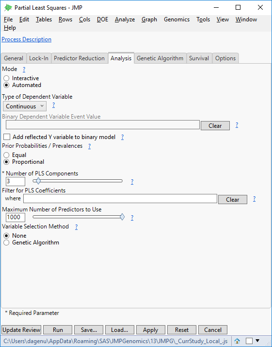
- Highlight the Partial Least Squares model and click Edit to bring up a settings window. There are several options available for survival, reducing predictors, and locking in variables. For this example, open the Analysis. Set the Type of Dependent Variable to Continuous.
- Set the Maximum Number of Predictors to Use to 1000. This will limit the number of markers allowed to make a prediction.
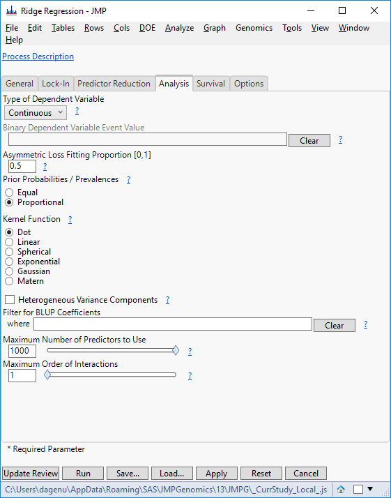
- Click Update Review to return to the original Predictive Modeling Review window. Select Ridge Regression, and on the Analysis tab, set the Type of Dependent Variable to Continuous and the Maximum Number of Predictors to Use to 1000.
- Again, click Update Review to return to the original Predictive Modeling Review window. Select Partition Trees now, and on the Analysis tab, set the Type of Dependent Variable to Continuous and click Update Review.
- The next three tabs give options for evaluating and comparing the models. We will use Cross Validation, but options are present for a Test Set if present and for Learning Curves.
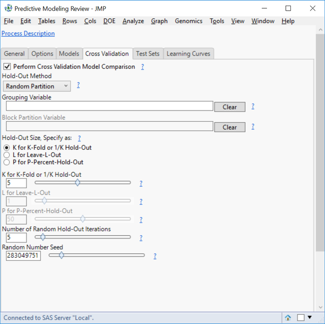
- In the Cross Validation tab, click the box next to Perform Cross Validation Model Comparison.
- For the Hold-Out Method, select Random Partition. This will randomly split the data into groups and then hold out a fraction of data from each group.
- Specify the Hold-Out Size as K for K-Fold and set the K for K-Fold slider to 5.
- Here, K is equal to the number of groups in a partition where 1/K equals the percentage of the total observations to hold out.
- Set the Number of Random Hold-Out Iterations to 5 to run the cross validation process 5 times for each model.
- Click Run to begin the analysis.
Results
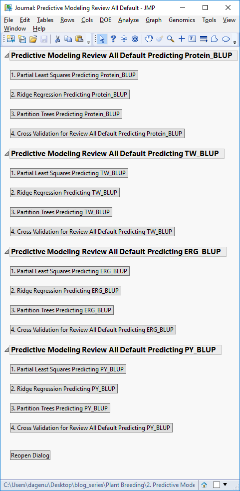
- When the analysis is finished, a JMP Journal window will appear with options for viewing each individual model’s results separated by the four traits, along with the results of the cross-validation model comparison.
- The results are organized by phenotype, with detailed results for how each model performed in predicting each trait. For the model comparison statistics, click the fourth result window for each trait, starting with Cross Validation for Review All Default Predicting Protein_BLUP.
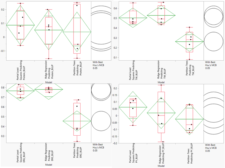
- The Cross Validation results include multiple methods for evaluating model effectiveness including RMSE, Harrel’s C, and Reliability Diagrams. We will asses the models based on Correlation. Higher correlation values are indicative of a more effective model. Each dot on the correlation plot represents one of the five cross validation iterations for each of the three model types. The correlation plots for each of the traits is shown below:
- Note that the axes of the four plots are different. According to this assessment, our Partial Least Squares and Ridge Regression models do a good job predicting Test Weight (TW) and Ergosterol Content (ERG). None of the models give an accurate prediction of Protein Content or Protein Yield (PY).
- The Ridge Regression model is slightly more effective at predicting TW and ERG, so we will select this model for cross evaluation. Before continuing, we will need to search the Output Folder where the results of the analysis are stored and find the Scoring Code Files for the ridge regression model. These files are SAS Program files named sas and barley_impu_PY_BLUP_02_rr_score.sas.
Summary
The Predictive Modeling Review in JMP Genomics is a one-stop-shop for fitting and comparing multiple models to your data. In this example, we fit four model types, each with unique settings. Note that multiple iterations of the same model type with differing settings can be included in the same review (i.e. a general linear model with LASSO vs. stepwise selection). Note that models can also be fit individually and tested against holdout data by selecting a model type from the Genomics Starter menu. Also note that fitting models individually may give more detailed output. The results of this analysis were two-fold: First, the knowledge that the Ridge Regression model is the most effective for predicting our phenotypes and second, a scoring code file which we will used as the basis for next week’s analysis, Cross Evaluation and Progeny Simulation with JMP Genomics, Part 3: Cross Evaluation, Selection, and Progeny Simulation.
- © 2026 JMP Statistical Discovery LLC. All Rights Reserved.
- Terms of Use
- Privacy Statement
- Contact Us


You must be a registered user to add a comment. If you've already registered, sign in. Otherwise, register and sign in.