- New to JMP? Let the Data Analysis Director guide you through selecting an analysis task, an analysis goal, and a data type. Available now in the JMP Marketplace!
- See how to install JMP Marketplace extensions to customize and enhance JMP.
JMP Blog
A blog for anyone curious about data visualization, design of experiments, statistics, predictive modeling, and more- JMP User Community
- :
- Blogs
- :
- JMP Blog
- :
- Why design experiments? Reason 6: Parsimony
- Subscribe to RSS Feed
- Mark as New
- Mark as Read
- Bookmark
- Subscribe
- Printer Friendly Page
- Report Inappropriate Content
I want to demystify design of experiments (DoE) with simple explanations of some of the terms and concepts that can be confusing for people when they are starting out. Throughout this series of blog posts, we have been using a case study where the objective is to understand how to set the Large Volume Injector (LVI) in a GC-MS analysis for trace impurities in water samples. We introduced an experimental plan that consists of testing 26 combinations of settings of the eight LVI factors as an example to illustrate some of the most important properties that we look for in a designed experiment.
In earlier posts in this series, we introduced multiple linear regression, and we saw that our 26-run experiment has useful correlation properties for understanding important behaviours including main effects, quadratic effects and two-factor interactions. However, we also revealed that it will not be possible to build a multiple linear regression model with all potentially important effects. We need a minimum of one run per effect in our model, and adding all the main effects, quadratics and two-factor interactions as well as the intercept, we counted a total of 44 parameters to estimate. We likened this to inviting 20 people to a meeting in a room that only seats 12.
In this post, we will see how we can understand which of all the possible effects are important for us to include our model. Einstein is attributed with saying that “everything should be made as simple as possible, but no simpler.”[1] This is the balance that we are aiming for here. We want a model of the system that captures the behaviours we need to know about so we can set the LVI to maximise our detection signal. We don’t want to miss important effects, but we don’t want an unnecessarily complex model either. We need a parsimonious model.
We will look at how we can use the data from our 26-run experiment to build a multiple linear regression model with just the most important effects. First, let’s return to the meeting analogy and hopefully not stretch it beyond breaking point!
Building the best meeting in steps

We will answer this using stepwise selection of attendees, starting at step 0.
Step 0. We start with nobody in the meeting room.
Step 1. We try each of the 20 people in the meeting on their own and keep the one person who results in the best quality of meeting: Katie – she is THE best person for this meeting. Everyone else is outside the room for now.
Step 2. Now we go through the remaining 19 possible attendees and put each of them in the room to find out which pair of Katie + 1 gives us the best meeting. We find that Katie + Robert is best. The other 18 are outside the room.
Step 3. We go through the remaining 18 attendees and find out which combination of Katie + Robert + 1 is best. We add Judy to the room.
Step 4. And so on…
Step 12. …until we have a full room.
Is this the best meeting that we can have? We found that Michael was the best person to add as the 12th attendee (the other eight were awful, especially Phillip). Will Michael contribute enough to the meeting to justify his inclusion? Will he just spend most of the time disrupting the meeting by tapping on his phone? Do we really need all 12 people in the meeting?
Now we look at how the quality of the meeting changed from steps 0 to 12. We look for where the meeting quality was highest and find it was at Step 4.
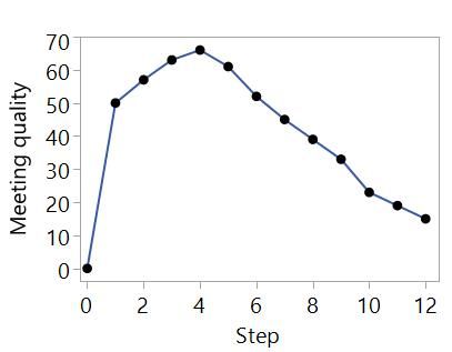
We conclude that the best meeting is with Katie, Robert, Judy and Louise. We have found the best balance that covers the understanding that we need for the meeting. Each of the other possible attendees could make a useful contribution, but it is not significant enough to outweigh the negative of having so many people in the room talking over each other.
Is this a good way to design a meeting? I'm not sure. Maybe you can try it and let me know. However, it is a good analogy for how we can build models using data from designed experiments.
Building the best model in steps
For the PkHt(SUM) model, we have the 44 possible effects. We will decide on our model in the same way as we decided who we should have in our meeting.
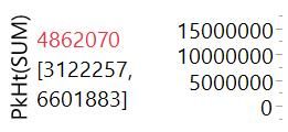
Step 0. We start by fitting an intercept-only model to the data from our 26-run experiment. Unless none of our factors have any important effect on the response, this model is too simple to be useful. The Prediction Profiler has no X-axes because we have no factor effects in the model:
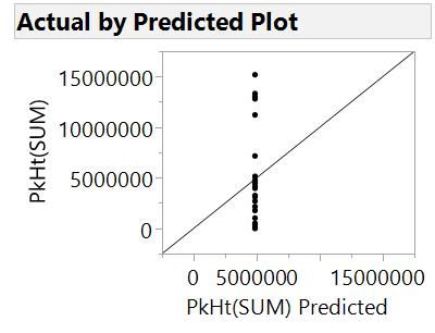
A plot of the actual response results versus the model prediction shows us that the model is not very useful.
There is poor agreement between the actual results for each run and the model predictions for those settings of that factors. The points would align to the 45-degree line for a model that predicts perfectly. The current model only predicts one value. It tells us the average PkHt(SUM) across all runs (4862070), which is the best estimate of what PkHt(SUM) will be if we know nothing about the effects of the factors.
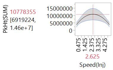
Step 1. We look for the best model that has the intercept and one of the other 43 parameters. We fit the 43 different possible models, and find that the model with the intercept and the quadratic effect of Speed(Inj) is the best. All 42 other effects are not in the model at this stage.
Here is the Profiler plot showing the curvilinear change in PkHt(SUM) with respect to Speed(Inj):
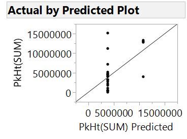
The actual versus predicted is improved but still not great:
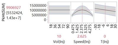
Step 2. We find that the interaction of Vol(Inj) and T(Inj) is the best effect to add at this step. We can see this effect from the Profiler plot with Vol(Inj) set at the lowest setting…
…and at the highest setting.
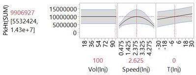
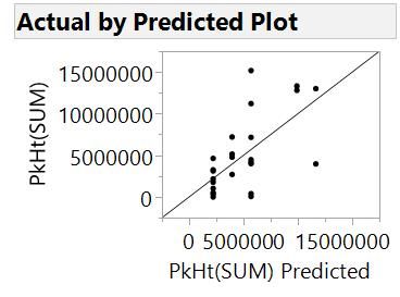
Notice how the slope for PkHt(SUM) versus T(Inj) changed. Again, agreement between actual and predicted is improved.
Steps 3 to 19. We go on in this way, adding the most important effect at each step.
Step 20. Fast forward to Step 20, and effects from all factors are included in a complex model with 20 effects plus the intercept.
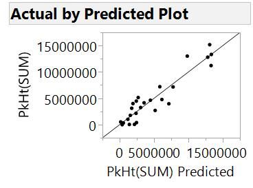
The actual versus predicted looks much better now.
We could go further until we have fit as many parameters as we have runs in the experiment, but we have probably overfit at this stage already. Now we look back at how model quality changed from steps 0 to 20. We can look at how the actual versus predicted has changed.
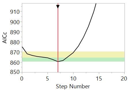
We can see that the model has improved as we progress through the steps, although maybe at the cost of complexity. At each step, we added the effect that resulted in the best model, but we didn’t say what “best” means. To have a process for deciding on the best model at each step and the best model over all steps, we need to be able to put a number on how good a model is. In fact, statisticians have thought up many ways to do this. In this example, we have used the corrected Akaike's Information Criterion or AICc. At each step, we added the effect that gave the model with the lowest AICc. Here, we have a plot of AICc versus step number:
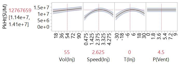
A lower AICc represents a better model: AICc reduces as the fit to the data improves; adding parameters to the model increases AICc. We can use it to find the sweet spot that balances goodness-of-fit and complexity. In this case, we see that AICc reduces from Step 0 to Step 7 and then increases off-the-scale towards Step 20. (The yellow and green bands are a guide -- models with an AICc in those ranges are somewhat equivalent to the best model.) We might therefore choose the model at Step 7:
Stepping forwards and backwards
The process we have described is called stepwise regression or stepwise selection. More specifically, we used forward stepwise selection. You could use backward selection when you have more runs than parameters to fit, so you can start with all the effects in the model and work backwards by taking out the least important effect at each step. You can also use a combination of forward and backward. Another choice you have is whether to specify effect heredity, so that second order effects can only be included if their main effects are also in the model. Models that obey effect heredity are generally preferred.
These various options and others are available in an automated stepwise process in software like JMP. The Generalized Regression platform in JMP Pro gives an interactive and visual interface to explore the model possibilities. This is useful because the final choice of model will rely not just on AICc or any one statistical measure.
“All models are wrong…
…But some are useful.”[2] This famous quote captures a truth that is worrying if you are new to DoE: There is no right answer at the end of it all! The model will approximate the real behaviour, so will always be “wrong” in some sense. You shouldn’t think that this is a problem. Models that are “wrong” in this way allow us to focus on understanding the important behaviours to meet our scientific and engineering objectives. As we said before, we are aiming for a parsimonious model.
With this example, we have seen how we can build useful models by sorting through a relatively large number of possible effects to find the important few. We have also seen how we can use statistical methods, along with our experience and knowledge of the system, to choose the most useful model. Our designed experiment gave us the data we needed to achieve this, and with the minimum experimental effort. At each step, the method can select the best effect because of the clarity that comes with the correlation properties of the design. Again, the take-home message is that if you want to be confident about efficiently getting to the most useful solution, you need to use DoE.
In the final post in this series, we will try to summarise all that we have learned and also talk about what we have missed.
Notes
[1] In fact, it seems that Einstein didn't say this. Ironically, his version was not as simple as it could have been.
[2] George Box. See this wikipedia entry for more.
- © 2026 JMP Statistical Discovery LLC. All Rights Reserved.
- Terms of Use
- Privacy Statement
- Contact Us



You must be a registered user to add a comment. If you've already registered, sign in. Otherwise, register and sign in.