- New to JMP? Join us Sept. 23-24 for the Early User Edition of Discovery Summit, tailor-made for new users. Register now for free!
- Learn some foundational elements of JMP Scripting Language (JSL) and how to extend point & click automation into repeatable, shareable routines. Register. June 26, 2 p.m. US Eastern Time.
JMP Blog
A blog for anyone curious about data visualization, design of experiments, statistics, predictive modeling, and more- JMP User Community
- :
- Blogs
- :
- JMP Blog
- :
- The QbD Column: A QbD factorial experiment
- Subscribe to RSS Feed
- Mark as New
- Mark as Read
- Bookmark
- Subscribe
- Printer Friendly Page
- Report Inappropriate Content

Editor's note: This post is by @ronkenett, Anat Reiner-Benaim and @david_s of the KPA Group. It is part of a series of blog posts called The QbD Column. For more information on the authors, click the authors' community names above.


A quick review of QbD
The first blog post in this series described Quality by Design (QbD) in the pharmaceutical industry as a systematic approach for developing drug products and drug manufacturing processes. Under QbD, statistically designed experiments are used to efficiently and effectively investigate how process and product factors affect critical quality attributes. They lead to determining a “design space,” a collection of production conditions that reliably provide a quality product.
A QbD case study
In this post, we present a QbD case study that focuses on setting up the design space. In this case study, the formulation of a steroid lotion of a generic product is designed to match the properties of an existing brand using in-vitro tests. In-vitro release is one of several standard methods that can be used to characterize performance of a finished topical dosage form. Important changes in the characteristics of a drug product formula (or the chemical and physical properties of the drug it contains) should show up as a difference in the drug release profile. A plot of the amount of drug released per unit area (mcg/cm2) against the square root of time should yield a straight line. The slope of the line represents the release rate, which is formulation-specific and can be used to monitor product quality. The typical in-vitro release testing apparatus has six cells in which the tested generic product is compared to the brand product. A 90% confidence interval for the ratio of the median in-vitro release rate in the generic and brand products is computed and then expressed as a percentage. If the interval falls within the limits of 75% to 133.33%, the generic and brand products are considered equivalent.
Initial assessment
An initial risk assessment maps the risks in meeting specifications of critical quality attributes (CQA). Table 1 presents expert opinions on the impact of manufacturing process variables on various CQAs. Cooling temperature was considered to have low impact; the order of ingredient addition was determined by considering the risk of contamination. Later, these two factors were not studied in setting up the process design space.
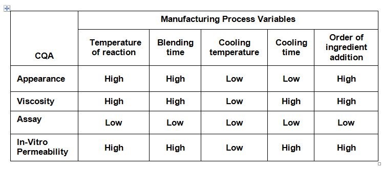
Table 1: Risk assessment of manufacturing process variables
The responses that will be considered in setting up the process design space include eight quality attributes:
- Assay of active ingredient.
- In-vitro permeability lower confidence interval.
- In-vitro permeability upper confidence interval.
- 90th percentile of particle size.
- Assay of material A.
- Assay of material B.
- Viscosity.
- pH values.
Three process factors are considered: temperature of reaction, blending time, and cooling time.
The experiment
To elicit the effect of the three factors on the eight responses, the company used a full factorial experiment with two center points. (See Table 2, which presents the experimental array in standard order.)
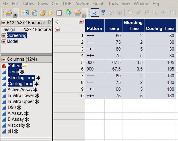
Table 2: Full factorial design with two center points
The JMP Prediction Variance Profile is useful to study the properties of the design. It shows the ratio of the prediction variance to the error variance, also called the relative variance of prediction, at various factor level combinations (Figure 1). Relative variance is minimized at the center of the design. As expected, if we choose to use a half-fraction replication with four experimental runs on the edge of the cube, instead of the eight-point full factorial, the variance will double.
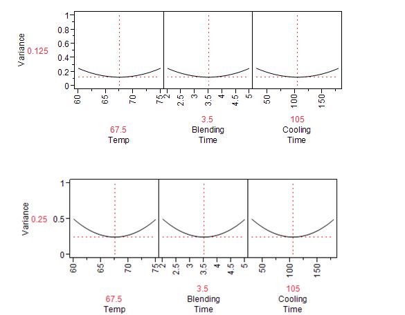
Figure 1: Prediction variance profile for full factorial design of Table 1 (top) and half-fraction design (bottom)
Conclusions about the factor effects
Each response is analyzed separately. Using the analysis of viscosity as an example, we see that the target value was 5000 and that results outside the range 4000-5600 were considered totally unacceptable. The 10 experimental results, shown in Figure 2, ranged from 4100 to 5600.
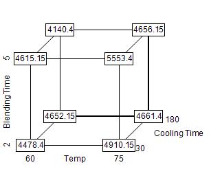
Figure 2: Cube display of viscosity responses
The strongest effect was associated with temperature, which was positively correlated with viscosity. However, none of the effects achieved statistical significance at the 5% level. (See Table 3)
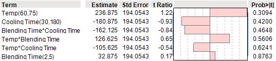
Table 3: Analysis of viscosity using second order interaction model
The case for center points
The two center points in the experimental array allow us to test for nonlinearity in the response surface by comparing the average responses at the center points (which for viscosity is 4135.5) to the average of the responses on the corners of the cube (in this case, 4851.6). We can obtain a formal significance test of nonlinearity by adding an “indicator” column – which has the value 1 for the center points and 0 for all other points – to the spreadsheet in Figure 2.
Combining all the response variables
The goal is to map out a design space that simultaneously satisfies requirements on eight responses: Active Assay, In-Vitro Lower, In-Vitro Upper, D90, A Assay, B Assay, Viscosity, pH. To achieve this objective, we apply a popular solution called the desirability function (Derringer and Suich, 1980), which combines the eight responses into a single index. For each response, Yi(x), i = 1, . . . , 8, the univariate desirability function di(Yi) assigns numbers between 0 and 1 to the possible values of Yi, with di(Yi) = 0 representing a completely undesirable value of Yi, and di(Yi) = 1 representing a completely desirable or ideal response value.
The desirability functions for the eight responses are presented graphically in Figure 3. For Active Assay, we aim to be above 95% and up to 105%. Assay values below 95% yield desirability of 0, assays above 105% yield desirability of 1. For In-Vitro Upper we do not want to be above 133%. Our target for D90 is 1.5 with results above 2 and below 1 having zero desirability. The design space can be assessed by an overall desirability index using the geometric mean of the individual desirabilities: Desirability Index = [d1(Y1) ∗ d2(Y2) ∗ . . . dk(Yk)] 1/ k with k denoting the number of measures (in our case k = 8). Notice that if any response Yi is completely undesirable (di(Yi) = 0), then the overall desirability is zero. From Figure 2 we can see that setting Temp=65, Blending Time=2.5 and Cooling Time=150 gives us an overall Desirability Index=0.31.

Figure 3: Prediction Profiler with individual and overall desirability function and variability in factor levels: (JMP) temp=65, blending time −2.5, cooling time −150
How variation in the production conditions affects desirability
JMP allows us to study the consequences of variability in the factor levels. Based on past experience, the production team was convinced that the inputs would follow independent normal distributions about their target settings, with standard deviations of 3 for Temp, 0.6 for Blending Time, and 30 for Cooling Time. Figure 3 shows how this input variability is transferred to the eight responses and to the overall desirability index via the statistical models from the experiments. JMP allows us to simulate responses and visualize how the variability in factor-level settings affects the variability in response. Viscosity and In-Vitro Upper show the smallest variability relative to the experimental range.
Finding the design space
To conclude the analysis, we applied JMP Contour Profiler to the experimental data, fitting a model with main effects and two-factor interactions. The overlay surface is limited by the area with In-Vitro Upper being above 133, which is not acceptable. As a design space, we identified operating regions with blending time below 2.5 minutes, cooling time above 150 minutes, and temperature ranging from 60-75 degrees Celsius. Once approved by the regulator, these areas of operations are defined as the normal range of operation. Under QbD, operating changes within this region do not require preapproval, only post-change notification. This change in regulatory strategy is considered a breakthrough in traditional inspection doctrines and provides significant regulatory relief for the manufacturer.
Monitoring production quality
An essential component of QbD submissions to the FDA is the design of a control strategy. Control is established by determining expected results and tracking actual results in the context of expected results. The expected results are used to set up upper and control limits as well as present the design space (see Figure 4). A final step in a QbD submission is to revise the risk assessment analysis. At this stage, the experts agreed that with the defined design space and an effective control strategy accounting for the variability presented in Figure 3, all risks in Table 1 have been reset as low.

Figure 4: Contour Profiler in JMP with overlap of eight responses
References
- Derringer, G., and Suich, R., (1980), Simultaneous Optimization of Several Response Variables, Journal of Quality Technology, 12, 4, 214-219.
- Kenett and Zacks, Modern Industrial Statistics with Applications in R, MINITAB and JMP, Wiley, 2014.
You must be a registered user to add a comment. If you've already registered, sign in. Otherwise, register and sign in.
- © 2026 JMP Statistical Discovery LLC. All Rights Reserved.
- Terms of Use
- Privacy Statement
- Contact Us