Structural equations models: A favorite amongst those who use them ... wonder why?

[#1]

If you’re in the behavioral or social sciences, chances are you know or have heard about structural equations models (SEM). The more experience folks have in these fields, the more likely they are to list SEM as their tool of choice. Why is that?

If you’re looking for a brief intro to SEM that helps you understand why this tool is highly valued amongst those who use it, then this blog post is for you. And if you’re an SEM expert, then this blog post might be a good resource to explain to your peers what it is you do (and why you love it so much!). Here are the ABCs of SEM.

Statistical Models = Path Diagrams

A central feature of SEM is that all models can be expressed with a path diagram. Consider the equations versus the diagram in Figure 1. If you must explain your statistical model to a 6-year-old, which of these versions do you prefer?

Figure 1. Equations versus path diagram representation of associations between W, X, and Y variables.

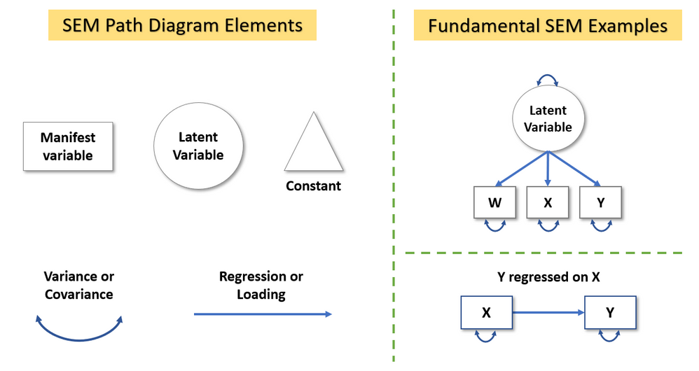
SEM users appreciate the intuitive nature of path diagrams, which enable them to convey their models effectively to wide audiences. Thus, we must start by describing how to create path diagrams correctly. The building blocks required for drawing path diagrams are in the left of Figure 2, and two standard path diagrams of SEM are depicted to the right of Figure 2.

Figure 2. Building blocks for drawing SEM path diagrams (left) and two examples of simple SEM models (right).

Here are the key guidelines for creating and interpreting path diagrams:

• Variables that you measure directly, are called “manifest” variables in SEM jargon and are drawn with squares.
• Unobserved variables or “latent” variables are factors in the factor analytic sense. That is, they represent the common variance across their manifest variables (aka indicators) and they cause the variation we observe in their indicators. Latent variables are represented with circles.
• A triangle is used to represent a constant, which is part of SEM to enable estimation of means and intercepts (regress a variable on a constant, and you get its mean). When models don’t place restrictions on variable means, the triangle is often omitted.
• One-headed arrows represent regression effects or loadings (loadings are regressions of a manifest variable on a latent variable).
• Double-headed arrows represent variances when they start and end on the same variable, and they represent covariances when they start and end on different variables.

Using these guidelines, you can draw path diagrams that specify highly complex models (picture the model in Figure 1 where W, X, and Y are all latent variables and additional predictors and outcomes are included)! The capacity to model relations among latent variables is why SEM is often thought of as a combination of factor analysis and regression.

The first model depicted on the right side of Figure 2 is a one-factor confirmatory factor analysis. Here, the latent variable has arrows pointing to W, X, and Y because the observed variation in these variables is caused by the latent variable. Note that latent and observed variables have a variance. However, to estimate such model one must set a scale for the latent variable. This is often done by fixing a loading or the latent variable’s variance to one. The second model depicted on the right side of Figure 2 is a simple regression. Note that X has a variance and it’s thus assumed to be normally distributed. This assumption is not made in the standard least squares regression. Yet, if we have missing data, making this assumption enables us to retain all available data in our analysis –a huge advantage of SEM!

Path Diagrams = Structure on Data

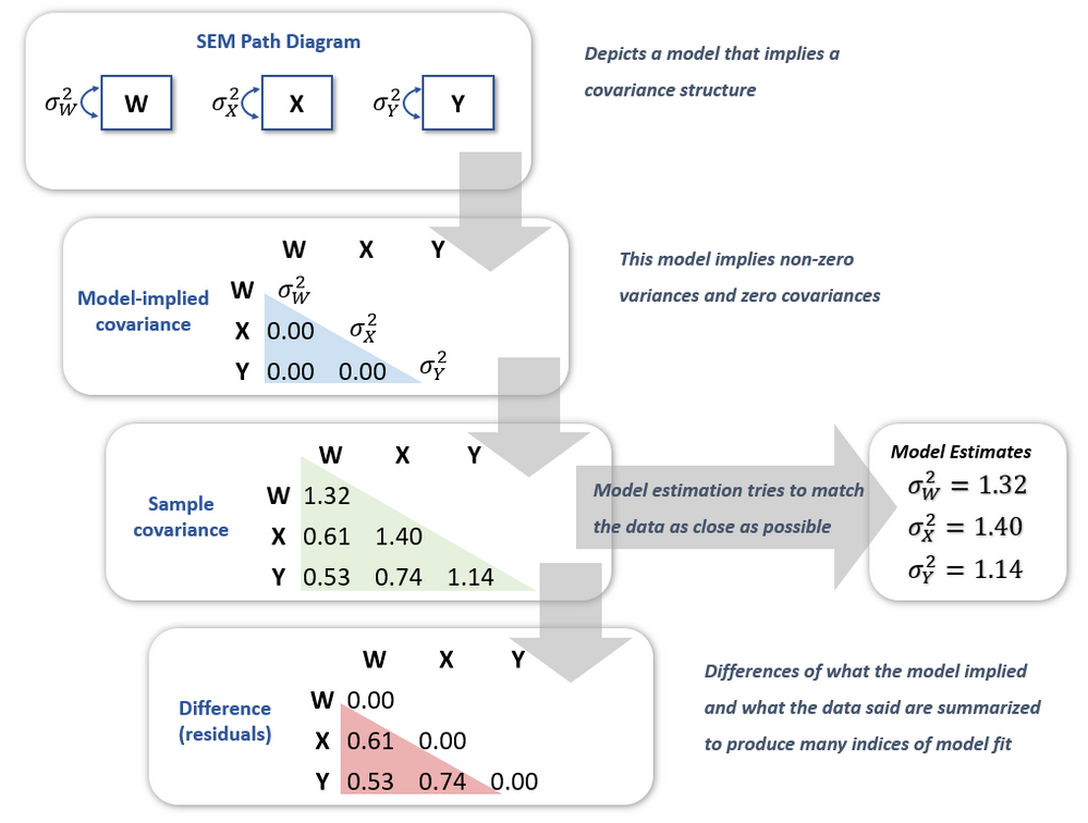
Another central feature of SEM is that path diagrams imply a specific structure on how variables covary. For example, the path diagram in the top box of Figure 3 has no connections linking any of the W, X, and Y variables. Thus, it implies that these variables are perfectly uncorrelated. Yet, the double-headed arrows indicate the variables have a non-zero variance. The next box in Figure 3 shows the implications of the path diagram on the covariance structure of the data. Indeed, the covariance matrix implied by the model shows three parameters for the variances and zeroes everywhere else.

Figure 3. Estimation of structural equations models; from path diagram to assessment of model fit.

Naturally, the data we collect have their own covariance matrix. Because we assume our data are multivariate normal, this matrix (and sometimes the variables’ means, but I’m leaving that for another post) is sufficient for our needs. Indeed, the sample covariance matrix is our best estimation of the population covariance matrix. Thus, estimation algorithms in SEM try to match the values in the sample covariance matrix as best as possible while retaining the constraints implied by the model. In Figure 3, the model implies three non-zero values for the variances of W, X, and Y, and thus, the model’s estimates are exactly the values of the diagonal in the sample covariance matrix.

Lastly, we can gauge the fit of the model by comparing the sample covariance matrix to the estimated model covariance matrix. The difference between these matrices (last box in Figure 3) gives us the model’s residuals, which can be normalized and summarized into fit indices that quantify the fit of the model. Note these residuals are unique to SEM, in that they're differences between sample and estimated covariances rather than between responses and predicted values, as in standard regression models.

Figure 3 captures the essence of SEM with a very simple example. The structure path diagrams can impose on the data can be much more complex but if Figure 3 makes sense, then you’re well on your way to understanding SEM!

Key Reasons for Using SEM

SEM is particularly useful if you have any of the following needs:

• Model variables that cannot be measured directly (aka latent variables)
• Model variables that have measurement error (and account for it)
• Specify a model in which variables are both predictors and outcomes
• Test specific theories about the association of variables
• Handle missing data with cutting edge methods without the hassle of multiple imputation
• Diagrams that describe your models intuitively

If you don’t relate to any of these needs, then SEM might not be ideal for your analyses. Indeed, just like there are lots of great reasons to use SEM, there are others that should discourage you from using this framework.

Key Reasons Not to Use SEM

SEM should not be used when analysts do not have a theory, or set of competing theories, that aim to explain patterns in the data. Research on automatic model searches for SEM is ongoing, but standard software does not implement the specialized algorithms arising from that work. Thus, to avoid type I errors (see MacCallum, Roznowski, & Necowitz, 1992), analysts should carefully devise their models ahead of time based on theory and previous research. This is particularly important to avoid confirmation bias.

If you’re comfortable fitting a regression model to a small sample (say, N = 30), then you can be equally comfortable fitting the equivalent regression model in SEM. However, with more complex models, analysts must consider whether their sample size is adequate. The number of variables, their distributions, missing values, and effect sizes play a role on determining adequate sample size (hint: there’s no simple rule of thumb!). Some research points to 5-10 observations per parameter estimate (Bentler & Chou, 1987), but even this might be misinformed when effect sizes are low or variables are skewed.

Variety of Models in SEM

SEM can be used for a range of purposes: from fitting a simple linear regression, to modeling a nonlinear process over time with factors that predict and are outcomes of that process. Other applications might involve:

• Developing a test or survey for measuring one or many latent variables through confirmatory factor analysis
• Testing mechanisms by which a set of variables lead to other variables through path analysis
• Investigating the indirect effect that one or many variables have on others through mediation analysis
• Characterizing individual and average trajectories of processes through latent growth curve analysis
• Studying dynamics within and between time series processes through dynamic factor analysis

Recommendations

Despite the simple and intuitive nature of path diagrams, SEM can be a highly complex technique. Thus, if you’re looking to learn more about this modeling framework, here are some references to get you started:

Excellent book with an applied focus:

Kline, R. B. (2016). Principles and practice of structural equation modeling (4th ed.). New York: Guilford Press.

Excellent book with technical details and applications:

Bollen, K. A. (1989). Structural Equations with Latent Variables. Wiley.

If you don’t have time for a whole book, try searching for this article with a general overview of SEM:

Ullman, J. B., & Bentler, P. M. (2013). Structural equation modeling. In J. A. Schinka, W. F. Velicer, & I. B. Weiner (Eds.), Handbook of psychology: Research methods in psychology (pp. 661-690). Hoboken, NJ, US: John Wiley & Sons Inc.

Ready to fit your own SEM? Check out this post to learn why the SEM platform in JMP Pro 15 will make your life easy!