- User Community
- :
- Blogs
- :
- JMP Blog
- :
- Self-organizing maps

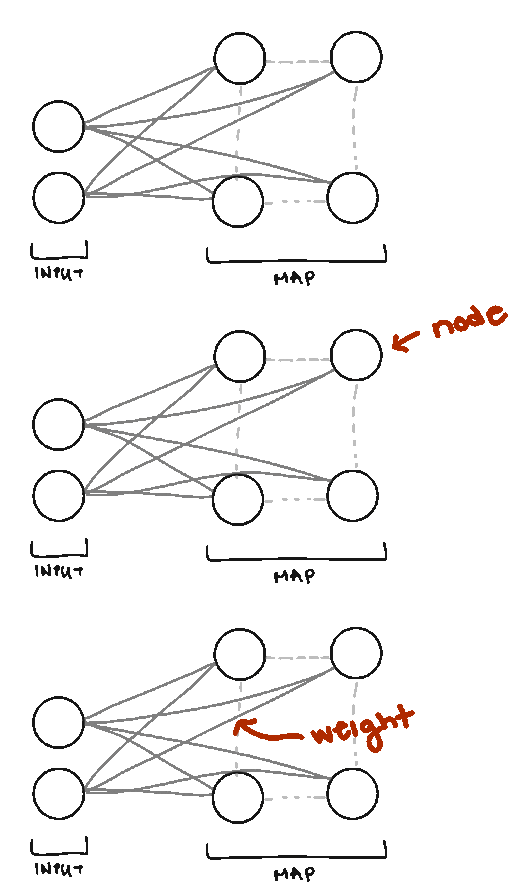
Traditionally, SOMs are explained as a form of Artificial Neural Network where features are inputs and clusters are outputs. But pretty much everything about how a SOM is trained and structured is different from traditional feedforward neural networks, even though some of the terms are the same. So if you’re starting with a blank slate Neural Network wise, you’ll still be able to follow this.
To make things easier, I’ll define some terms and what they mean up front:
Node. We call them nodes because we’re borrowing terms from Neural Networks, but the nodes in SOMs represent the centers of each of our clusters. The number of nodes you have is the number of clusters you’ll have.
Weight. We also borrow the term weight from Neural Networks, but the weights in SOMs are different. Weights represent the spatial position of the node (like how in K-Means we have cluster centers). The weights will be the same dimension as our data vectors.
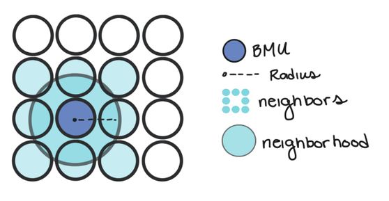
Neighborhood. The neighborhood of a node is all the nodes that are sufficiently close to it. How close is “sufficiently” close will change as we train our SOM.
Learning Rate. The learning rate reflects how much we’ll change our node weights on each iteration. Large learning rates mean our weights might fluctuate wildly. Very small learning rates means our weights won’t change much from their initial values.
Lattice/Map. The arrangement/grid of nodes in our Map.
Incremental-Learning SOM
To give you a better general idea of what SOMs do, we will start by looking at SOMs that are trained iteratively, which will let us see each step in the SOMs creation one by one. This isn’t the method that JMP implements. To be computationally efficient, JMP trains its SOMs with the batch method, which we will see below.
Overview. There are five main steps to train a SOM iteratively:
- Initialize the weights of the SOM nodes. This can either be done randomly, or particular starting weights can be chosen so that they are spread out efficiently across all possible input values (which JMP does).
- Choose a random data point from your data set.
- Calculate which Node the data point is closest to. We can do this by calculating the distance between our data point and each node weight. The node that is the closest is called the Best Matching Unit (BMU for short).
- Once we know the BMU, we calculate which nodes are in the neighborhood of the BMU. In other words, which nodes are sufficiently close in the map to the BMU.
- We update the weight of the BMU and all of its neighbors so that their weights are more similar to our data point. Essentially, we’re making our clusters fit better with our data. Nodes that are further from the BMU are changed less than nodes near to the BMU (and the BMU itself).
We repeat steps 2-5 until we’ve reached our maximum number of iterations, or our node weights stop changing.
In Depth. Let’s take a deeper look at steps 3-5 to understand what’s going on more intuitively.
Before we start, don’t let the math keep you from reading this section. I’m going to show you formulas, but it’s OK if you don’t understand all the math, as long as you know the general idea behind why we use this math.
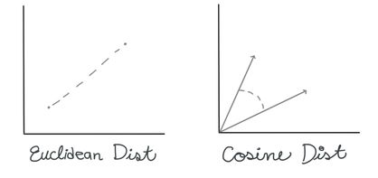
Finding the BMU. There are many ways you can calculate the distance between two n-dimensional vectors; commonly with SOMs, you may see measures like Euclidean Distance or Cosine Distance.
In this case, we’re going to use the Euclidean distance. To calculate the BMU, we calculate the Euclidean distance between our selected data vector and each of the weight vectors for our nodes. The BMU has the smallest distance.
Calculating neighborhoods. Updating multiple nodes/cluster centers separates SOMs from simpler methods like K-Means. Not only will we change the weight of our BMU to be closer to the data vector, but we’re also going to change nodes that we think are sufficiently close to the BMU.
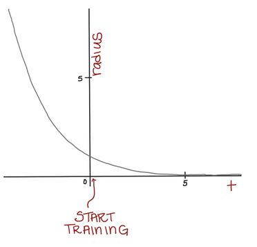
Nodes are considered in a BMU’s neighborhood if they’re within a certain radius of the BMU. In other words, if a node is inside a circle with radius, r, centered at the BMU, it’s considered a neighbor.
At first, we want to use a large-ish neighborhood and change many nodes. But, as time goes on, we want our neighborhoods to get smaller so we can do some more “fine-tuning” of our SOM. Think about how, when sanding something, we often start with large grit sandpaper and work our way down to finer grit sandpaper.
Mathematically, we can achieve this by using a formula for our neighborhood radius, r, that depends on time and gets smaller as we continue to train our SOM. Eventually, the neighborhood will be so small, it will only contain the BMU.
Updating node weights. Once we know which node weights we want to update, we calculate how much to change them. The weights of nodes closest to the BMU will change the *most*, and the nodes that are on the very edge of our neighborhood will change very little. But all node weights will be pulled closer to the current data vector.
We do so using this formula (don’t worry, I’ll walk you through the different parts in a moment):
The W’s represent the node weight. W(t+1) is our updated weight, W(t) is our current weight. If we simplify the latter part of the right-hand side for a moment, we can see that the new, updated weight is our old weight multiplied by some adjustment.
(V(t) - W(t)) is the distance between our data vector, and the current node weight. This shows that our adjustment is going to depend on how far apart the data vector and node are.
L(t) is the learning rate. Just like our neighborhood function (actually EXACTLY like our neighborhood radius function…), our learning rate starts out at a relatively large value, , and gets smaller over time (the exponential part does that for us.)
When we first start training our SOM, our learning rate is high, but over time we want our node weights to be more stable, so we decrease our learning rate.
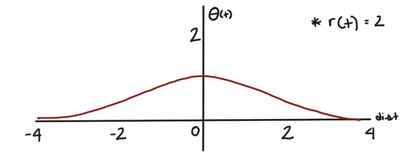
Not only is the learning rate decreasing over time, but the change to our node weights is also decreasing as the node gets further from our BMU. is a Gaussian kernel, which mathematically represents this decay. (dist is the distance between the node we’re changing and the BMU in the map.)
For a given radius, r(t), the Gaussian kernel will be this shape:
When the distance between the node we’re updating and the BMU is large, will be small. Conversely, when the node we’re updating is close to the BMU, will be larger.
We have finally deconstructed the whole formula!
To review:
W(t) is the current weight of a node.
causes nodes that are further from the BMU to be changed less than nodes close to the BMU (and the BMU itself).
L(t) is our decaying learning rate. As time goes on, we’re “fine-tuning” and making smaller changes than we are at the start of training.
V(t) - W(t) is the distance between the data vector and the node weight (both n-dimensional). The larger the distance, the more things will change.
If you’ve made it this far, you deserve a break! We’ve reviewed the way that SOMs are trained iteratively. This showed us the general ideas that make SOMs unique: namely the way we update multiple node weights depending on time, distance from the BMU, and distance between the data vector and the node weight.
If you’ve ever read about SOMs elsewhere, the thing people get excited about is that SOMs “preserve topology,” which is just a fancy way of saying that nodes that are close together in multi-dimensional space will be close together in our SOM grid once we’ve trained it. This helps us visualize our data using the SOM grid since it’s easy to graph things in two dimensions...but much harder in multiple dimensions.
Learning about iterative SOM training is useful for understanding these properties, but it’s not computationally efficient. That’s why JMP uses the batch training method to actually do the SOM calculations.
Batch Learning SOM
This algorithm is the one described in the JMP website. Instead of training our SOM one data vector at a time, we can use all the data vectors at once!
Here are the steps:
- Initialize the weights of the SOM nodes (this is the same in the iterative method)
- All at once, calculate the BMUs for each data vector in our training set.
- Compute the new node weights by using this formula:
is the number of data vectors whose BMU is node j,
is the mean of all those data vectors and is the neighborhood function which decides which nodes get changed, and by how much. It’s similar to the
in our incremental training algorithm.
4. Repeat 2 and 3 until our SOM has converged.
The math can be more difficult to follow when it happens all at once, but the basic premise of the Batch Learning algorithm is that instead of updating our nodes in response to one data vector, we update them in response to all the data vectors at once (sorta like K-Means…). And thankfully for you, this method will often speed up the time it takes for JMP to train your SOM.
In JMP
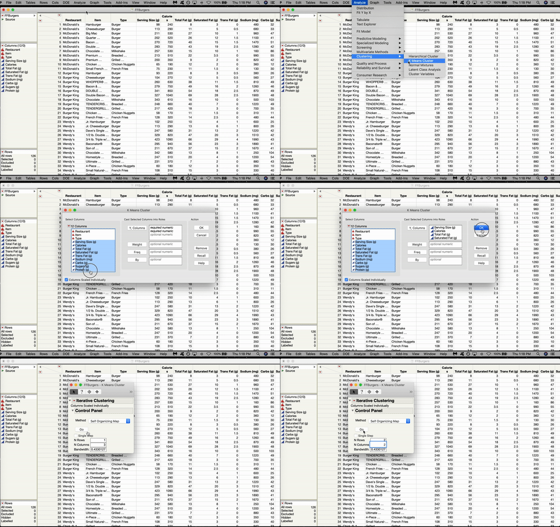
In JMP, the SOM option is located in the K-Means menu. Let’s use a SOM to cluster some Fast Food Hamburgers from various American restaurants. Go to Analyze > Clustering > K-Means. The K-Means Cluster window will pop up. Click and Drag all the variables you want to use over to the Y box and Click OK.
Inside the Control Panel, there’s a dropdown menu for Method. Choose Self Organizing Map. From here, you can choose the size of your grid. We’ll do 2x2, which gives us four nodes arranged in a rectangular shape. Click GO.
Our output automatically shows us the means of each of our four clusters. We can save these cluster assignments by going to the red triangle under our SOM Grid menu and selecting “Save Clusters”. In that same menu, we can also select “Biplot” to see a visual representation of our SOM. JMP will plot the nodes/clusters by the first two Principal Components. Here, it looks like Cluster 1 (at the top) is quite far from the other three. We can check that out later in Graph Builder.
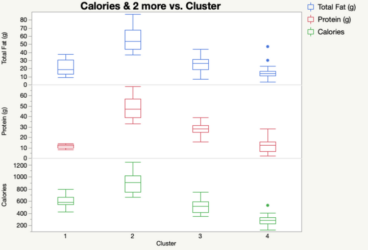
Even by examining a few of our variables, we can start to see why Cluster 1 was so different. It has absolutely NO protein. If we look at our data set, we can see that the items in Cluster 1 tend to be desserts.
Cluster 2, on the other hand, is high in Calories, Protein and Fat! You might want to watch out for those items if you’re looking to stay awake for long after you eat them.
Conclusion
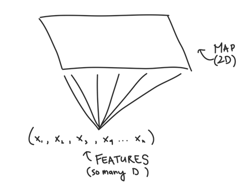
Self Organizing Maps are a useful tool to cluster your data by building a map that takes potentially highly dimensional data and mapping it into a much more manageable 2D form. In JMP, SOMs are just as easy to implement as K-Means (even if the math behind it is much more complicated), so what have you got to lose by trying them out?
You must be a registered user to add a comment. If you've already registered, sign in. Otherwise, register and sign in.
- Subscribe to RSS Feed
- Mark as New
- Mark as Read
- Bookmark
- Subscribe
- Printer Friendly Page
- Report Inappropriate Content
- © 2025 JMP Statistical Discovery LLC. All Rights Reserved.
- Cookie Preferences
- Terms of Use
- Privacy Statement
- Contact Us

