Predictive modeling is all about finding the model that accurately predicts the outcome of interest. Let’s say, for example, that I want to predict the progression of a particular disease – in this case, diabetes – after one year, based on a number of factors. More specifically, I want to identify patients who are most likely to have high disease progression so that appropriate interventions can be made.
I have JMP Pro, and I know that there are several possible predictive models I can fit. For example, I can fit a regression model, various types of tree-based models, or a neural network, to name a few. Which modeling platform should I use? Which type of model will predict the outcome most accurately? For any given modeling situation, the best model depends largely on the data – there’s no one type of model that works best for all problems.
To find the best model for the diabetes scenario, I can fit all of the possible models, one at a time, using cross-validation. I can save the individual models to the data table, or to the Formula Depot, and then use Model Comparison to compare the performance of the models on the validation set to select the best one. Or I can select the best combination of models. While this method more than gets the job done, it does require a bit of work.
Now, with the new Model Screening platform in JMP Pro 16, we’ve made this much easier. Model Screening provides an efficient workflow for simultaneously fitting, comparing, exploring, selecting and then deploying the best predictive model.
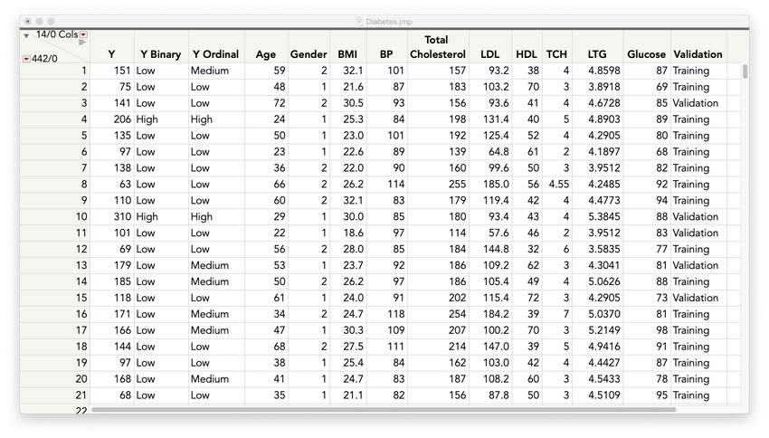
To illustrate, I’ll use the Diabetes data from the JMP Sample Data library. The response, or outcome variable, is Y Binary, which has two possible values: Low (for low disease progression) and High. The predictors, or factors, are Age through Glucose.
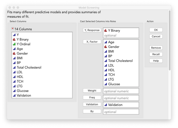
I select Model Screening from the Analyze > Predictive Modeling menu and specify the response and factors. The Validation column partitions the data into Training and Validation sets, so I’ll use this for model validation.
The top portion of the Model Screening dialog is shown here:
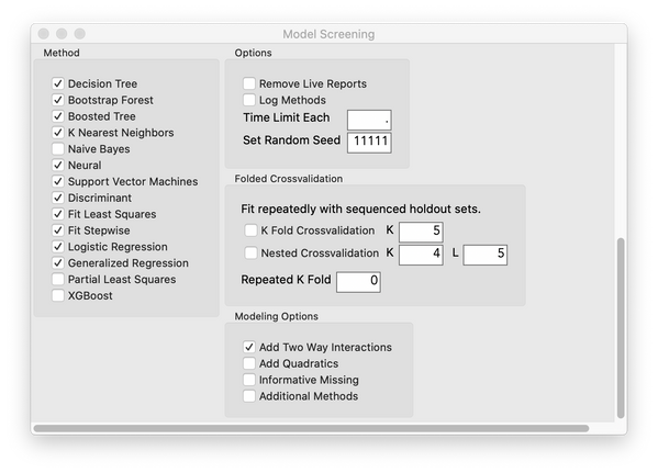
At the bottom of the dialog, there are several different modeling methods to choose from, along with many different fitting and cross-validation options. Note that XGBoost is an available method, because I installed the XGBoost Add-In from the JMP User Community.
I’ll use the default models, but will add two-way interactions and will set the random seed to 11111 to make my results reproducible.
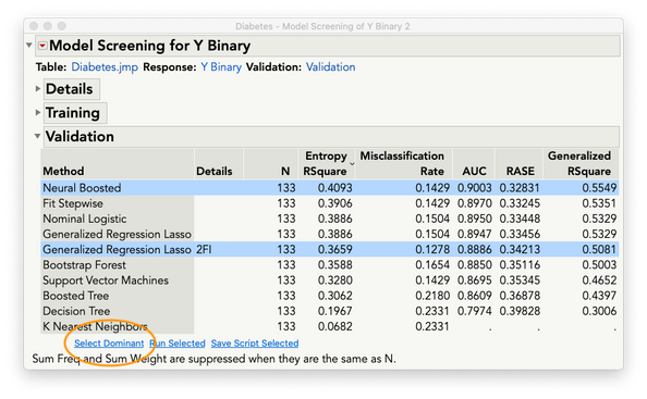
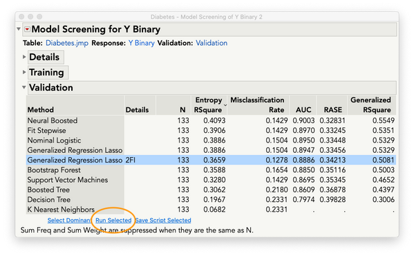
All of the models that make sense for these data are fit, and several validation statistics are provided. The models are sorted in descending order of Generalized RSquare, but to find the model or models that stand out across all of the validation statistics, I’ll click Select Dominant.
I can see that the top models, overall, are Neural Boosted and Generalized Regression Lasso with two-way interactions.
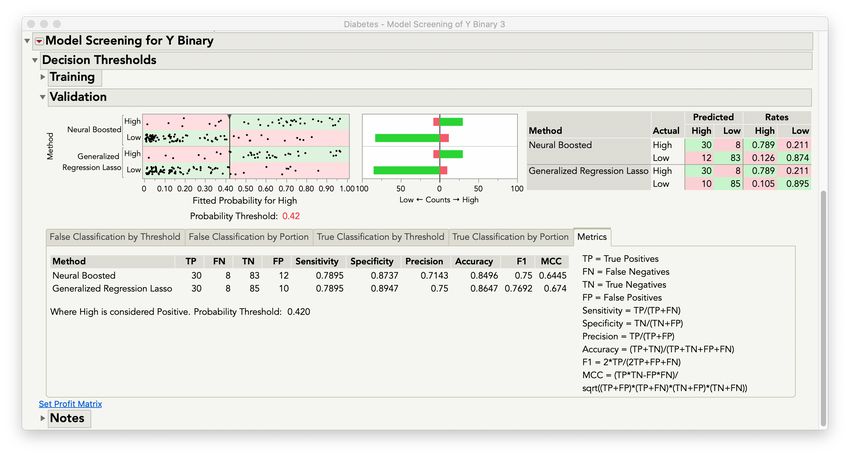
To explore the classifications for these models, I’ll select Decision Threshold from the top red triangle menu. This option provides a wealth of information for comparing the classification accuracy of the selected models. The top section shows the breakdown of true and false classifications for each model, and if I change the probability threshold (either by dragging the slider line or using the edit box), I can see how the classifications and classification errors change for different cutoffs.
The bottom section has tabs showing different classification graphs and metrics. The Metrics tab for the validation data is shown here. In this scenario, I want to identify patients who are most likely to have a high rate of diabetes progression. So, I want to find the model that results in the lowest false negative rate. At a probability threshold of 0.42, the Generalized Regression model has a low false negative rate, while still maintaining a low false positive rate relative to the other model.
Now, I might want to take a closer look at this model. Model Screening makes this seamless. I can easily run the selected model in a new window by clicking Run Selected.
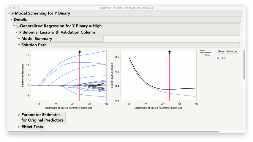
 Or, without leaving Model Screening, I can see the results directly in the Details outline as shown here. In Model Screening I have access to all of the options I'd see in Generalized Regression. So, for example, I can interact with the solution path, and I can save or publish the model for deployment. I can even run other models to see if I can get further improvement in model accuracy.
I've only touched the surface of Model Screening here, but hopefully you can see how this streamlined workflow can help you save a lot of time and effort! You simply need to specify the variables in your model, select the models you want to fit and the validation method, and Model Screening does the rest!
To learn more about fitting and validating predictive models in JMP Pro, go to the key features page at our website.
What Customers Say
"Having used model screening on JMP Pro 16 beta these past few months, it has already become an indispensable part of my coral reef predictive modeling research. Although models could be compared rather easily in earlier versions of JMP Pro (e.g., JMP Pro 15’s “model comparison” platform), this new tool makes it even easier for users to simultaneously test many different models (e.g., gen-reg, PLS, discriminant, neural networks, etc.) with the same data set. Something that once took me hours or even days can now be done in minutes (or even seconds). Wow, what a great feature! This surely must be the biggest improvement from version 15 to 16, and I’m sure many others will feel the same."
- Anderson Mayfield, National Oceanic and Atmospheric Administration (NOAA) and the University of Miami