Editor's Note: This post was written by @eric_cai, a chemist and statistician who also blogs at The Chemical Statistician. Follow Eric on Twitter @chemstateric.
One of the most common tasks in chemistry is to determine the concentration of a chemical in an aqueous solution (i.e., the chemical is dissolved in water, with other chemicals possibly in the solution). A common way to accomplish this task is to create a calibration curve by measuring the signals of known quantities of the chemical of interest - often called the analyte - in response to some analytical method (commonly involving absorption spectroscopy, emission spectroscopy or electrochemistry); the calibration curve is then used to interpolate or extrapolate the signal of the solution of interest to obtain the analyte's concentration.
However, what if other components in the solution distort the analyte's signal? This distortion is called a matrix interference or matrix effect, and a solution with a matrix effect would give a different signal compared to a solution containing purely the analyte. Consequently, a calibration curve based on solutions containing only the analyte cannot be used to accurately determine the analyte's concentration.
Overcoming Matrix Interferences with Standard Addition
An effective and commonly used technique to overcome matrix interferences is standard addition. This involves adding known quantities of the analyte (the standard) to the solution of interest and measuring the solution's analytical signals in response to each addition. (Adding the standard to the sample is commonly called "spiking the sample.") Assuming that the analytical signal still changes proportionally to the concentration of the analyte in the presence of matrix effects, a calibration curve can be obtained based on simple linear regression. The analyte's concentration in the solution before any additions of the standard can then be extrapolated from the regression line; I will explain how this extrapolation works later in the post with a plot of the regression line.
Procedurally, here are the steps for preparing the samples for analysis in standard addition:
1) Obtain several samples of the solution containing the analyte in equal volumes.
2) Add increasing and known quantities of the analyte to all but one of the solutions.
3) Dilute the mixture with water so that all solutions have equal volumes.
These three steps are shown in the diagram below. Notice that no standard was added to the first volumetric flask.

This above image was made by Lins4y via Wikimedia with some slight modifications.
At this point, the five solutions are now ready for analysis by some analytical method. The signals are quantified and plotted against the concentrations of the standards that were added to the solutions, including one sample that had no standard added to it. A simple linear regression curve can then be fitted to the data and used to extrapolate the chemical concentration.
Determining the Concentration of Silver in Photographic Waste: An Illustrative Example in JMP
The following example is from pages 117-120 in "Statistics for Analytical Chemistry" by J.C. Miller and J.N. Miller (2nd edition, 1988). The light-sensitive chemicals on photographic film are silver halides (i.e., ionic compounds made of silver and one of the halogens: fluorine, bromine, chlorine and iodine). Thus, silver is often extracted from photographic waste for commercial reclamation. A sample of photographic waste containing an unknown amount of silver was determined by standard addition with atomic absorption spectroscopy. Here are the data in JMP:
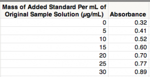
I used the "Fit Y by X" platform and the "Fit Line" option under the red-triangle menu to implement simple linear regression. (You can also do this with the "Fit Special" option; just click "OK" without adjusting any settings.) After adjusting the axes and adding some captions, I get the following plot:
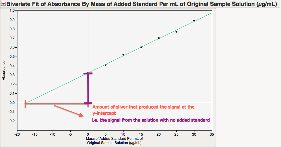
This plot illustrates the key idea behind using this calibration curve. The magnitude of the x-intercept is the concentration of the silver in the original solution. To understand why this is so, consider the absorbance at the following two values:
- at x = 0, the value of y is the absorbance of the solution with no added standard (i.e., it corresponds to the concentration of silver that we ultimately want).
- at the x-intercept, there is no absorbance.
Thus, the magnitude of the difference between x=0 and the x-intercept is the concentration of silver that is needed to produce the signal for the original solution of interest! Our job now is to determine the x-intercept.
Using a little linear algebra, we can mathematically obtain the x-intercept. However, there is a clever way to find it in JMP using the "Inverse Prediction" function under "Fit Model". (I thank @Mark_Bailey, another JMP blogger, for his guidance on this trick!)
First, let's run the linear regression again by "Fit Model" under the "Analyze" menu.
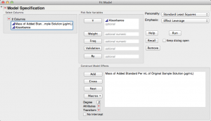
Notice how JMP automatically suggests "Standard Least Squares" in the top right of this dialog window.
Here is the output from "Fit Model".
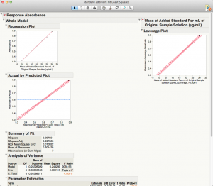
Now, to get the x-intercept, let's go to the red-triangle menu for "Response Absorbance." Within the "Estimates" sub-menu, choose "Inverse Prediction." This allows us to predict an x-value given a y-value. Since we need the x-intercept, the y-value (absorbance) needs to be zero. I prefer to use a significance level of 1%, so I set my confidence level at 0.99.

There is an option on the bottom left that says "Confid interval with respect to individual rather than expected response," and you may be wondering what it means. This option allows you to get the prediction interval, which quantifies how certain I am about the x-value (silver concentration) of a new observation at "Absorbance = 0". In contrast, a confidence interval quantifies how certain I am about the mean silver concentration at that particular absorbance. A prediction interval takes into account two sources of variation:
- Variation in the estimation of the mean x-value.
- Variation in the sampling of a new observation.
A confidence interval takes only the first source of variation into account, so it is narrower than a prediction interval.
Since I am interested in the x-intercept alone and not a new observation at zero absorbance, let's leave that option unchecked and just use a confidence interval.
Here is the output that has been added to the bottom of this results window.
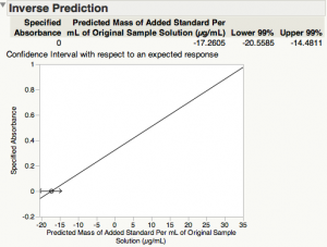
The estimate of the x-intercept (concentration of silver in the standard solution at zero absorbance) is 17.2605 µg/mL, and its 99% confidence interval [14.4811, 20.5585].
Conclusion
Standard addition is a simple yet effective method for determining the concentration of an analyte in the presence of other chemicals that interfere with its analytical signal. Its use of simple linear regression can be easily implemented and visualized in JMP using the "Fit Model" platform, and its "Inverse Prediction" function provides an easy way to not only estimate the analyte's concentration, but also to generate a confidence interval for it.
References
J.C. Miller and J.N. Miller. Statistics for Analytical Chemistry. 2nd Edition, 1988, Ellis Horwood Limited. Pages 117-120.
G. Gruce and P. Gill. "Estimates of Precision in a Standard Addition Analysis." Journal of Chemical Education, Volume 76, June 1999.
Eric Cai works as a Data Science Consultant at Environics Analytics in Toronto, Canada. He shares his passion about statistics, machine learning, chemistry and math via his blog, The Chemical Statistician; his YouTube Channel; and his Twitter feed @chemstateric. This is Eric's first post as a guest blogger for JMP.