In this blog post, Sr. Analytics Software Tester @Mark_Bailey and I explain a few new features in JMP Pro 17. The JMP development team has worked hard to build into the software new chemometric analysis capability. Most of the new capability centers around Functional Data Explorer. Now, with a few mouse clicks, you can preprocess your curve data, save the preprocessed data to a new table for further multivariate analysis, and complete a functional analysis of this data in one platform. We will focus on analyzing spectral data in this post, but please note that this platform analyzes virtually any of your chemometric data with outstanding results.
Many thanks to @clay_barker, @RyanParker, and @chris_gotwalt1 for pulling this chemometric analysis capability into one platform.
Preprocessing
Preprocessing spectral data couldn’t be much easier than with FDE. There is a new Spectral tab where you will find several pre-processing tools, including Standard Normal Variate (SNV), Multiplicative Scatter Correction (MSC), Savitzky-Golay smoothing with 1st and 2nd derivative capability, and Baseline Correction.

Figure 1. Screen Shot of New Pre-processing Capability Built into FDE
We demonstrate the newer chemometric analysis capability in JMP Pro using a near-infrared data set from Dyrby et al., Applied SpectroscopyVol 56, Number5, 2002.
Initial Pre-processing
For this data set, the initial preprocessing steps were SNV followed by Baseline Correction. The Baseline Correction was a quadratic model over the entire function. You can see in the images below how the preprocessing worked to mitigate most of the variation in the data.
Use a single preprocessing method or use them in combination to get the most out of your data standardization. One of the more common combinations seen in many scientific articles is to take the Savitzky-Golay 1st Derivative and then take the SNV for a final step. This combination works well, but do not be shy about trying several combinations to see what works best for your data.


Figure 2. Tablet NIR Data Before and after pre-processing
Save the preprocessed data as a new stacked table for further multivariate analysis steps. You should transpose the data back to the wide format for any additional analyses.
Wavelet Modeling
We previously showed how to use B-Splines and P-Splines in FDE to model spectral data. With JMP Pro 17, a new Wavelet modeling capability is added primarily for chemometric data. You’ll find the new Wavelet model toggle under the red triangle (Functional Data Explorer > Models > Wavelets).
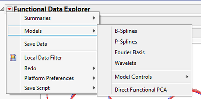
Figure 3. Models associated with FDE in JMP Pro 17
Wavelet modeling is much better at fitting curve data with many peaks than either of the spline methods.
The Wavelet model output, as seen below, quickly fits the data for all 310 batches. The result suggests that a Symlet 4 model fits all of the data the best out of 15 other algorithms based on the Bayesian Information Criteria (BIC). The model with the lowest BIC is the best.
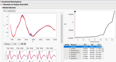
Figure 4. Wavelet Model Selection and Best Fit Based on BIC
Because FDE finds the best model for the shape of the curve of interest, you see that the Functional Principal Components (FPC) are now called Shape Functions.

Figure 5. New Shape Function Designation for FDE Data
You can also see that the Eigenvalue plot still shows how much the individual shape functions explain shape variation.
At this point, you will want to save the Function Summaries to a new table. Click the red triangle for Function Summaries and select Save Summaries. The Functional Principal Components will be saved with the Wavelet coefficients to this new table with your supplementary variables. We will revisit this table in the Predictive Modeling section.
A new Control Chart Builder function also graphs the Function Summaries by the FPCs for each sample ID.
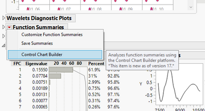
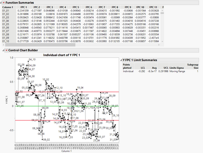
Figure 6. Control Chart Builder Built into FDE.
As before, you can limit the number of components used to define the shape by using the FPCA Model Selection tool. This reduction will help simplify your model when most of the variation is explained by a smaller number of shape components than shown in the original model.
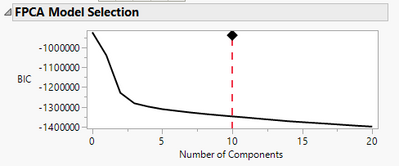
Figure 7. Functional Principal Component (Shape Function) Model Selection Tool
Wavelets DOE Analysis
The last new function is Wavelets DOE Analysis, which is found in the red triangle menu for Wavelets (Wavelets on Reduce Grid (404)).
Transformations are very fast with data on a grid. The reduced grid ensures the wave numbers are evenly spaced, with no decimal points. JMP develops the reduced grid for you, but you can control how regular the grid is if you choose.
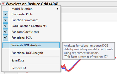
Figure 8. Wavelet DOE Selection Option.
For this data, we want to see which curve or set of curves best emulates a given percent API. The Wavelet coefficients are quickly analyzed using the Generalized Regression platform. The resulting Wavelet DOE Profiler is used to find the wavelength or set wavelengths that define the differences between the various percentage levels. Because the coefficients represent wavelengths and resolutions, they are used to build a more interpretable model than what may have been possible using FPCs.
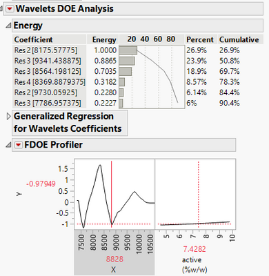
Figure 9. Wavelet DOE Energy Graphic and FDOE Profiler.
In the image above, the Energy table shows the most significant differences for all coefficients. The coefficient for Res 2 at wavelength 8175 has the highest energy, representing about 27% of the total energy of the active wavelengths. As a bonus, the coefficients directly represent specific wavelengths or peaks in the curve data.
Building a Predictive Model from the Wavelet Coefficients
The new summaries table is useful for statistical analysis and predictive modeling. The FPCs could be used to build a predictive model, or another option is to build a predictive model based on a subset of the Wavelet coefficients data using the Generalized Regression platform. As you can see in the table margin below, there is a column for all 512 Wavelet coefficients. Likely, you will only need a small subset of all the coefficients to build a good predictive model.
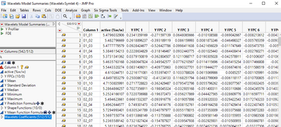
Figure 10. Wavelet Model Summaries Table (512 Coefficients).
The Generalized Regression model below shows the fit using all of the Wavelet coefficients data as variables for the fit. Elastic Net penalization was used with Elastic Net Alpha of 0.56 to include as many essential wavelengths as possible but to avoid overfitting by using all 512 Wavelet coefficients in the model.
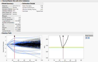
Figure 11. Generalized Regression Model Fit.
Try the new techniques with your own data sets or ask us for a demonstration. Thanks again to our excellent development team, and we look forward to hearing your feedback on these game-changing enhancements to the software.