- Subscribe to RSS Feed
- Mark Topic as New
- Mark Topic as Read
- Float this Topic for Current User
- Bookmark
- Subscribe
- Mute
- Printer Friendly Page
Discussions
Solve problems, and share tips and tricks with other JMP users.- JMP User Community
- :
- Discussions
- :
- Re: how to compare oscilloscope traces and detect outlier traces?
- Mark as New
- Bookmark
- Subscribe
- Mute
- Subscribe to RSS Feed
- Get Direct Link
- Report Inappropriate Content
how to compare oscilloscope traces and detect outlier traces?
Hello,
i am wondering if there is a way in JMP to compare oscilloscope voltage traces to tell whether the traces are statistically the same or different.
the reason i want to know is bc i collect example scope traces to qualify power supplies. when i plot the traces they visually appear to line up quite well (both the waveform shape and voltage magnitudes), but of course the traces aren't identical. i am wondering if there is a comparison method to identify outlier scope traces.
my traces are square or pulsewidth type waveforms, which plot voltage vs. time
thanks!
- Mark as New
- Bookmark
- Subscribe
- Mute
- Subscribe to RSS Feed
- Get Direct Link
- Report Inappropriate Content
Re: how to compare oscilloscope traces and detect outlier traces?
Based on your comment regarding how well they visually line up, the first question I must ask is when you look at the graphs are they practically significantly different? How much of a change in the graphs would matter to you? There are many ways to quantify the plots (e.g., max, min, slope, amplitude). You can use any of those as response variables and test for differences.
- Mark as New
- Bookmark
- Subscribe
- Mute
- Subscribe to RSS Feed
- Get Direct Link
- Report Inappropriate Content
Re: how to compare oscilloscope traces and detect outlier traces?
And what do you have, a picture or a data table? I'm guessing you get a .CSV table from the scope.
Are you looking at periodic data? Are you looking for timing of pulses? Or maybe low-level noise? Or sharp corners on square waves?
I think different tools could be designed for different concerns.
- Mark as New
- Bookmark
- Subscribe
- Mute
- Subscribe to RSS Feed
- Get Direct Link
- Report Inappropriate Content
Re: how to compare oscilloscope traces and detect outlier traces?
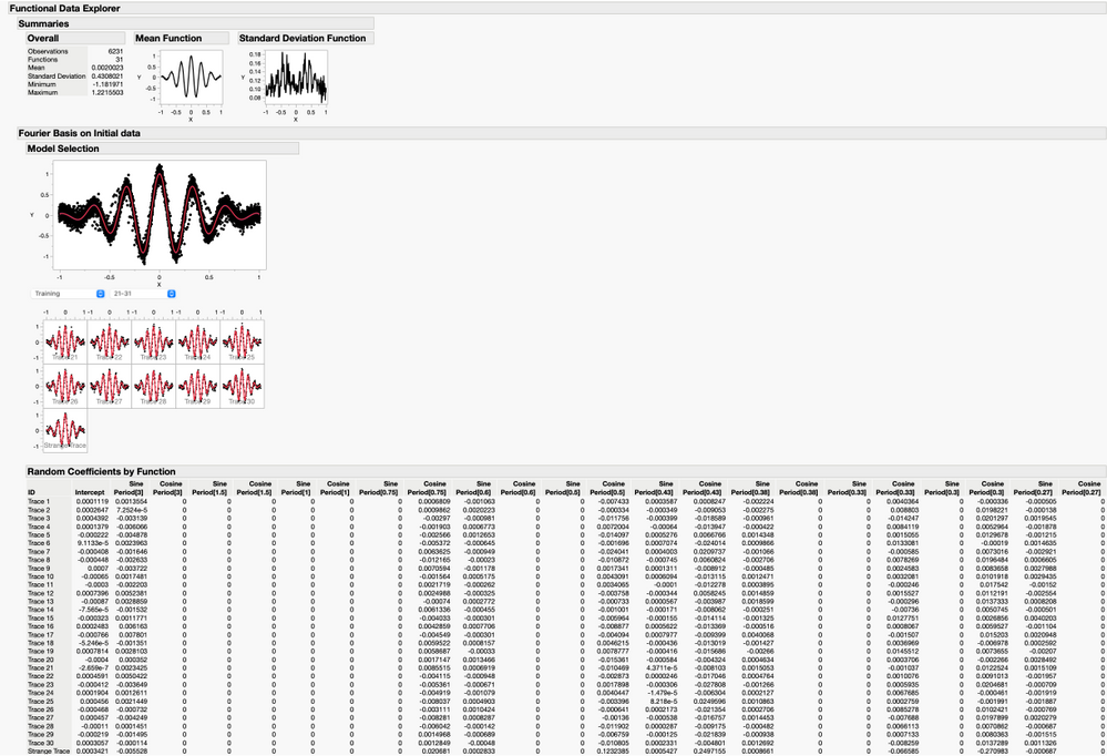
Here is an idea that uses Functional Data Explorer in JMP Pro. FDE can do Fourier decomposition in a easy way, and you can look at the Fourier basis coefficients to see if any of them look unusual compared to the rest.
// find unusual signal trace idea
Names Default To Here( 1 );
// create some signal traces, with one trace that is different from the others
ntraces = 30;
npoints = 100;
points = (-1 :: 1 :: .01)`;
npoints = N Rows( points );
noise = 0.1;
traces = [];
For( ii = 1, ii <= ntraces, ii++,
	trace = Cos( 2 * Pi() * 3 * points ) :* Exp( -Pi() * points ^ 2 )
	+J( npoints, 1, Random Normal( 0, noise ) );
	traces = traces || trace;
);
strangetrace = Cos( 2 * Pi() * 2.5 * points ) :* Exp( -Pi() * points ^ 2 )+J( npoints, 1, Random Normal( 0, noise ) );
traces = traces || strangetrace;
// put them into a data table and name columns descriptively
dt = As Table( points || traces );
dt << Set Name("Example Traces");
Column( dt, 1 ) << Set Name( "X" );
For( ii = 1, ii <= ntraces, ii++,
	Column( dt, ii + 1 ) << Set Name( "Trace " || Char( ii ) )
);
Column( dt, ntraces + 2 ) << set name( "Strange Trace" );
// graph the traces
dt << Graph Builder(
	Size( 534, 454 ),
	Show Control Panel( 0 ),
	Variables(
		X( :X ),
		Y( :Trace 1 ),
		Y( :Trace 2, Position( 1 ) ),
		Y( :Trace 3, Position( 1 ) ),
		Y( :Trace 4, Position( 1 ) ),
		Y( :Trace 5, Position( 1 ) ),
		Y( :Trace 6, Position( 1 ) ),
		Y( :Trace 7, Position( 1 ) ),
		Y( :Trace 8, Position( 1 ) ),
		Y( :Trace 9, Position( 1 ) ),
		Y( :Trace 10, Position( 1 ) ),
		Y( :Trace 11, Position( 1 ) ),
		Y( :Trace 12, Position( 1 ) ),
		Y( :Trace 13, Position( 1 ) ),
		Y( :Trace 14, Position( 1 ) ),
		Y( :Trace 15, Position( 1 ) ),
		Y( :Trace 16, Position( 1 ) ),
		Y( :Trace 17, Position( 1 ) ),
		Y( :Trace 18, Position( 1 ) ),
		Y( :Trace 19, Position( 1 ) ),
		Y( :Trace 20, Position( 1 ) ),
		Y( :Trace 21, Position( 1 ) ),
		Y( :Trace 22, Position( 1 ) ),
		Y( :Trace 23, Position( 1 ) ),
		Y( :Trace 24, Position( 1 ) ),
		Y( :Trace 25, Position( 1 ) ),
		Y( :Trace 26, Position( 1 ) ),
		Y( :Trace 27, Position( 1 ) ),
		Y( :Trace 28, Position( 1 ) ),
		Y( :Trace 29, Position( 1 ) ),
		Y( :Trace 30, Position( 1 ) ),
		Y( :Strange Trace, Position( 1 ) )
	),
	Elements(
		Line(
			X,
			Y( 1 ),
			Y( 2 ),
			Y( 3 ),
			Y( 4 ),
			Y( 5 ),
			Y( 6 ),
			Y( 7 ),
			Y( 8 ),
			Y( 9 ),
			Y( 10 ),
			Y( 11 ),
			Y( 12 ),
			Y( 13 ),
			Y( 14 ),
			Y( 15 ),
			Y( 16 ),
			Y( 17 ),
			Y( 18 ),
			Y( 19 ),
			Y( 20 ),
			Y( 21 ),
			Y( 22 ),
			Y( 23 ),
			Y( 24 ),
			Y( 25 ),
			Y( 26 ),
			Y( 27 ),
			Y( 28 ),
			Y( 29 ),
			Y( 30 ),
			Y( 31 ),
			Legend( 5 )
		)
	)
);
// use FDE to find Fourier Basis Functions and Coefficients for Each Trace and save to a data table
Local( {obj},
	obj = dt <<
	Functional Data Explorer(
		Data Format( Column ),
		Y(
			:Trace 1, :Trace 2, :Trace 3, :Trace 4, :Trace 5, :Trace 6, :Trace 7,
			:Trace 8, :Trace 9, :Trace 10, :Trace 11, :Trace 12, :Trace 13,
			:Trace 14, :Trace 15, :Trace 16, :Trace 17, :Trace 18, :Trace 19,
			:Trace 20, :Trace 21, :Trace 22, :Trace 23, :Trace 24, :Trace 25,
			:Trace 26, :Trace 27, :Trace 28, :Trace 29, :Trace 30, :Strange Trace
		),
		X( :X ),
		Fourier Basis(
			Functional PCA(
				1,
				FPC Profiler(
					1,
					Confidence Intervals( 1 ),
					Term Value(
						X( 0, N Levels( 201 ), Lock( 1 ), Show( 1 ) ),
						FPC 1( 0, Lock( 0 ), Show( 1 ) )
					)
				)
			)
		),
		SendToReport(
			Dispatch(
				{"Functional Data Explorer"},
				"Data Processing",
				OutlineBox,
				{Close( 1 )}
			),
			Dispatch(
				{"Functional Data Explorer", "Fourier Basis on Initial data"},
				"Random Coefficients by Function",
				OutlineBox,
				{Close( 0 )}
			),
			Dispatch(
				{"Functional Data Explorer", "Fourier Basis on Initial data"},
				"Functional PCA",
				OutlineBox,
				{Close( 1 )}
			)
		)
	);
	Report( obj )["Fourier Basis on Initial data", "Random Coefficients by Function",
	Table Box( 1 )] << Make Into Data Table;
	obj << Close Window;
);

outdt= Get Data Table List()[1];
outdt << Set Name("Fourier Basis Coefficients for Traces");
// use explore outlier screening platform to find traces with outlying basis function coefficients
// note, this last step is specific to this problem, other problems might use more or less fourier basis
// functions, but the same general approach using Explore Outlier (Analyze > Screening > Explore Outliers)
// shoudl work fine

outdt << Explore Outliers(
	Y(
		:"Sine Period[3]"n, :"Cosine Period[3]"n, :"Sine Period[1.5]"n,
		:"Cosine Period[1.5]"n, :"Sine Period[1]"n, :"Cosine Period[1]"n,
		:"Sine Period[0.75]"n, :"Cosine Period[0.75]"n, :"Sine Period[0.6]"n,
		:"Cosine Period[0.6]"n, :"Sine Period[0.5]"n, :"Cosine Period[0.5]"n,
		:"Sine Period[0.43]"n, :"Cosine Period[0.43]"n, :"Sine Period[0.38]"n,
		:"Cosine Period[0.38]"n, :"Sine Period[0.33]"n, :"Cosine Period[0.33]"n,
		:"Sine Period[0.3]"n, :"Cosine Period[0.3]"n, :"Sine Period[0.27]"n,
		:"Cosine Period[0.27]"n
	),
	Robust Fit Outliers( Huber( 1 ) ),
	SendToReport(
		Dispatch( {"Robust Fit Outliers"}, "", TabListBox, {Set Selected( 2 )} )
	)
);
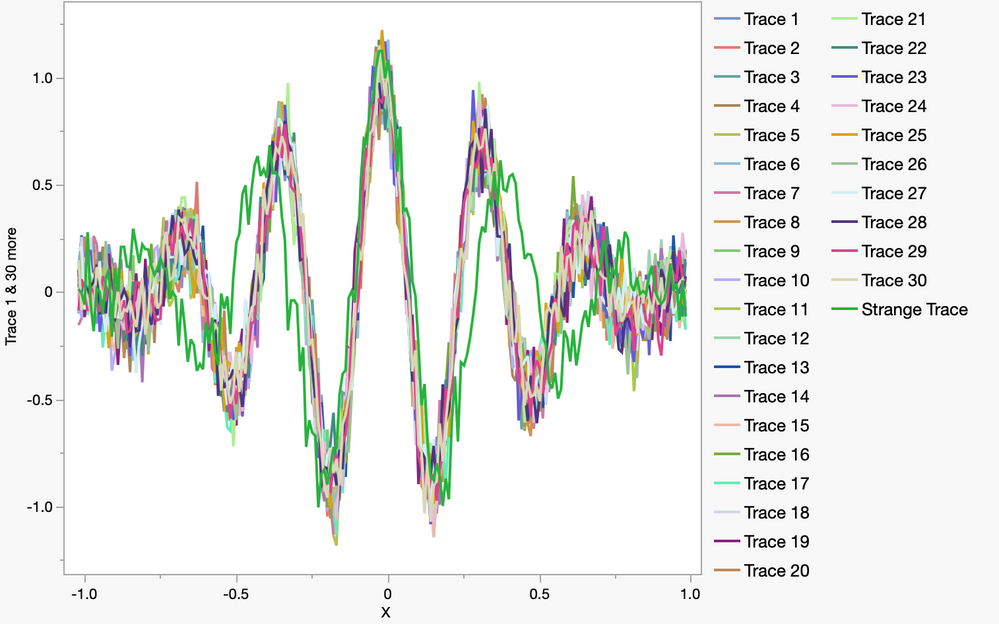
Example graph of generated traces (with added noise, one of the traces is different than all the others)
FDE output (summarized)
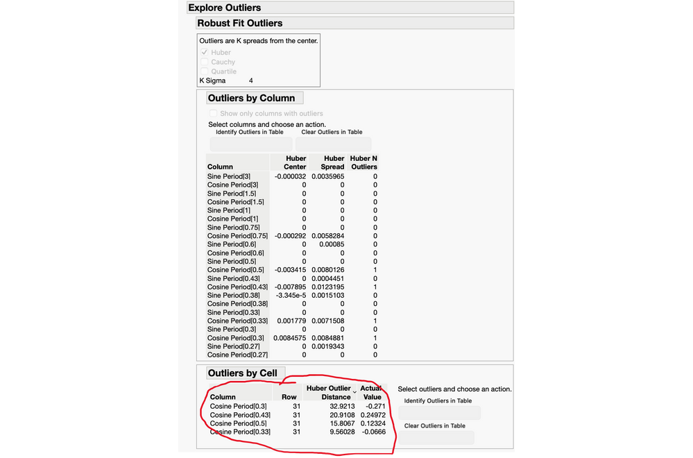
Explore Outliers detects the "Strange Trace" (Row 31) based on it's Fourier Basis coefficients
Recommended Articles
- © 2026 JMP Statistical Discovery LLC. All Rights Reserved.
- Terms of Use
- Privacy Statement
- Contact Us


