- New to JMP? Let the Data Analysis Director guide you through selecting an analysis task, an analysis goal, and a data type. Available now in the JMP Marketplace!
- See how to install JMP Marketplace extensions to customize and enhance JMP.
- Subscribe to RSS Feed
- Mark Topic as New
- Mark Topic as Read
- Float this Topic for Current User
- Bookmark
- Subscribe
- Mute
- Printer Friendly Page
Discussions
Solve problems, and share tips and tricks with other JMP users.- JMP User Community
- :
- Discussions
- :
- fit special polynomial - how to input coefficients?
- Mark as New
- Bookmark
- Subscribe
- Mute
- Subscribe to RSS Feed
- Get Direct Link
- Report Inappropriate Content
fit special polynomial - how to input coefficients?
Hi.
Im plotting data using Fit Y by X.
I would like to plot a pre-known quadratic as a reference line (rather than fitting one to the data shown). I can see how this would be done for a linear fit using Fit Special, linear, then constrain the intercept and slope to what ever values, but when selecting quadratic (or higher orders) from the drop down box it doesnt give you somewhere to input the extra coefficients to constrain.
Can I do it via script instead and if so what would the format be?
Many thanks
Accepted Solutions
- Mark as New
- Bookmark
- Subscribe
- Mute
- Subscribe to RSS Feed
- Get Direct Link
- Report Inappropriate Content
Re: fit special polynomial - how to input coefficients?
Hi,
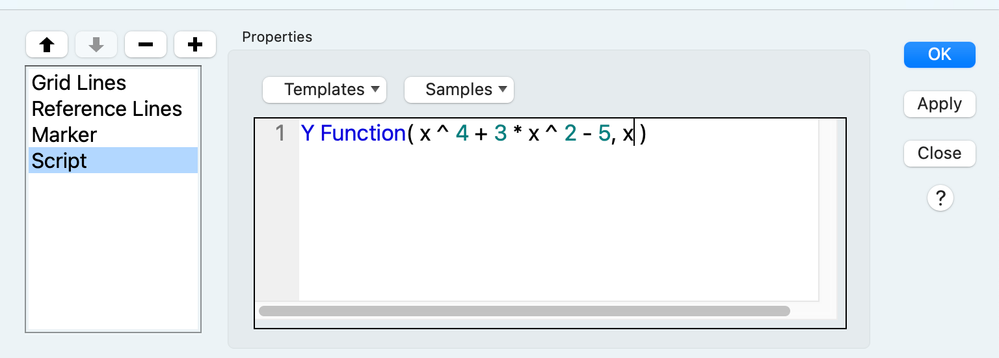
Right-clicking on the graph, select "Customize" from the context menu, click the "+" icon. From here you can add a script using the Y function ( ) function, which takes 2 arguments: an expression (the function) and the domain variable (here, x).
Click OK and you're done.
This is also easy to do via scripting with the Y function ( ) function. Here, y = 2x^2 + 3x -5, corresponding to coefficients [2, 3, -5] is plotted. I've used Horner's rule here, as it makes things easier in the next illustration.
dt = astable(J(40,2,randominteger(-20,20)));

gb = dt << Graph Builder( Variables( X( :Col2 ), Y( :Col1 ) ), Elements( Points( X, Y, Legend( 3 ) ) ) );

report(gb)[framebox(1)] << add graphics script ( Y Function( (2 * x + 3) * x - 5, x ) );
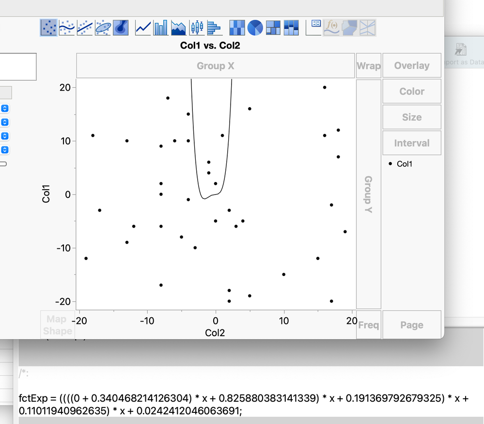
One issue is that the coefficients might be determined at runtime, might not be integers, and the degree of the polynomial might be unknown. In this case something like the following will work:
dt = astable(J(40,2,randominteger(-20,20)));

gb = dt << Graph Builder(
	Variables( X( :Col2 ), Y( :Col1 ) ),
	Elements( Points( X, Y, Legend( 3 ) ) ),
);

// get random uniform coefficient matrix
coef = J(5, 1, randomuniform());

// build an expression using Horner's rule:
for each ( {v, i }, coef,// i = 1; v = coef[i];
	if (i  > 1,
		fctExp = insert ( insert ( expr ( multiply ( ) ), nameExpr ( fctExp ) ), expr ( x ) );
	,
		fctExp = expr ( 0 );
	);
	fctExp = insert ( insert ( expr( add ( ) ), nameexpr( fctExp ) ), v );
);

// substitute into a graph script expressison and evaluate
graphAdd = expr (
	report(gb)[framebox(1)] << add graphics script ( Y Function( _EXPRESSION_ , x ) )
);

eval ( substitute ( nameexpr(graphAdd), expr( _EXPRESSION_ ), nameexpr ( fctExp ) ) );

//show the expression in the log
show ( fctExp )
- Mark as New
- Bookmark
- Subscribe
- Mute
- Subscribe to RSS Feed
- Get Direct Link
- Report Inappropriate Content
Re: fit special polynomial - how to input coefficients?
Hi,
A possible low-tech solution would be to compute your reference curve in a separate column in your data table and then plot it with the rest of the data.
Best,
TS
- Mark as New
- Bookmark
- Subscribe
- Mute
- Subscribe to RSS Feed
- Get Direct Link
- Report Inappropriate Content
Re: fit special polynomial - how to input coefficients?
Hi,
Right-clicking on the graph, select "Customize" from the context menu, click the "+" icon. From here you can add a script using the Y function ( ) function, which takes 2 arguments: an expression (the function) and the domain variable (here, x).
Click OK and you're done.
This is also easy to do via scripting with the Y function ( ) function. Here, y = 2x^2 + 3x -5, corresponding to coefficients [2, 3, -5] is plotted. I've used Horner's rule here, as it makes things easier in the next illustration.
dt = astable(J(40,2,randominteger(-20,20)));

gb = dt << Graph Builder( Variables( X( :Col2 ), Y( :Col1 ) ), Elements( Points( X, Y, Legend( 3 ) ) ) );

report(gb)[framebox(1)] << add graphics script ( Y Function( (2 * x + 3) * x - 5, x ) );
One issue is that the coefficients might be determined at runtime, might not be integers, and the degree of the polynomial might be unknown. In this case something like the following will work:
dt = astable(J(40,2,randominteger(-20,20)));

gb = dt << Graph Builder(
	Variables( X( :Col2 ), Y( :Col1 ) ),
	Elements( Points( X, Y, Legend( 3 ) ) ),
);

// get random uniform coefficient matrix
coef = J(5, 1, randomuniform());

// build an expression using Horner's rule:
for each ( {v, i }, coef,// i = 1; v = coef[i];
	if (i  > 1,
		fctExp = insert ( insert ( expr ( multiply ( ) ), nameExpr ( fctExp ) ), expr ( x ) );
	,
		fctExp = expr ( 0 );
	);
	fctExp = insert ( insert ( expr( add ( ) ), nameexpr( fctExp ) ), v );
);

// substitute into a graph script expressison and evaluate
graphAdd = expr (
	report(gb)[framebox(1)] << add graphics script ( Y Function( _EXPRESSION_ , x ) )
);

eval ( substitute ( nameexpr(graphAdd), expr( _EXPRESSION_ ), nameexpr ( fctExp ) ) );

//show the expression in the log
show ( fctExp )
- Mark as New
- Bookmark
- Subscribe
- Mute
- Subscribe to RSS Feed
- Get Direct Link
- Report Inappropriate Content
Re: fit special polynomial - how to input coefficients?
Your initial suggestion of adding a script via the customize function worked. Thank you!
Recommended Articles
- © 2026 JMP Statistical Discovery LLC. All Rights Reserved.
- Terms of Use
- Privacy Statement
- Contact Us


