- Subscribe to RSS Feed
- Mark Topic as New
- Mark Topic as Read
- Float this Topic for Current User
- Bookmark
- Subscribe
- Mute
- Printer Friendly Page
Discussions
Solve problems, and share tips and tricks with other JMP users.- JMP User Community
- :
- Discussions
- :
- distribution parameters mismatch between Competing Risk Mixture and SubSample in...

- Mark as New
- Bookmark
- Subscribe
- Mute
- Subscribe to RSS Feed
- Get Direct Link
- Report Inappropriate Content
distribution parameters mismatch between Competing Risk Mixture and SubSample in Life Data platform
Hi All,
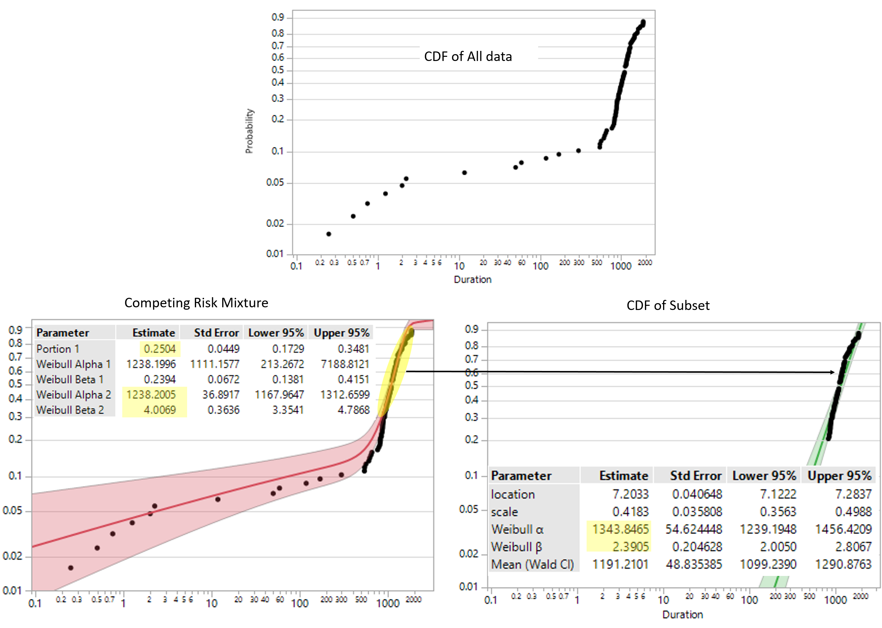
I use Life Distribution platform from Reliability and Survival to fit distribution to reliability results.
To distinguish between failure causes I used 2 Weibull distributions in Competing Risk Mixture of Life Distribution platform (see graphs below and attached file).
Portion 1 value (marked with yellow) from the Competing Risk Mixture report species part of reliability results related to 1st Weibull distribution.
In Life Distribution platform Weibull distribution was fitted to [ 1 - (Portion 1) ]% subset of reliability results.
As far as I understand Weibull parameters of 2nd distribution in Competing Risk Mixture report and subset have to match, but they are actually not (marked with yellow).
Why Weibull parameters between 2nd distribution in Competing Risk Mixture report and subset are different?

Accepted Solutions

- Mark as New
- Bookmark
- Subscribe
- Mute
- Subscribe to RSS Feed
- Get Direct Link
- Report Inappropriate Content
Re: distribution parameters mismatch between Competing Risk Mixture and SubSample in Life Data platform
What you did is not what I suggested. What you have done in the last using "Life Distribution - Compare Groups" is a third analysis in this thread of discussion. What you have done is technically identical to what you have done in your second analysis. That is why you get "same" results. I don't understand the objective, so I will stop trying to guide on your specific data. In the following, I will use JMP sample data sets to make my points, be useful in general to the audience who read this thread.
First, "Competing Risk Mixture" and "Competing Cause" are two different analyses. The terms "competing risk" and "competing cause" may be used interchangeably in the literature. They both take rows of observations, and each observation is a time-to-event observation. And each observation is associated with a cause. But in some experiments, you known the cause; in other experiments, you don't. When you don't have failure causes, you use Competing Risk Mixture. When you have failure causes, you use "Competing Cause". Competing Risk Mixture helps you to guess distributions of individual failure causes, but won't be able to tell the causes of individual observations for sure. Competing Cause fits distributions of individual failure causes, and failure cause is known information. Under normal use cases, there should not be confusion about which analysis to use, and one should not modify data in order to switch analysis types. "Appliance.jmp" is a sample data under Reliability sample data folder to illustrate Competing Cause. There is a Cause Code column in the table. The column "Y2" in "Mixture Demo.jmp", a sample data under Reliability sample data folder, is created to illustrate Competing Risk Mixture. There is no cause information in the table.
Second, when using Competing Cause, there is no need for user to modify data. The software modifies the data for the user to fit the model. Here is what the software does conceptually. I use "Appliance.jmp" as an example.
- For every cause code, create a copy of the entire data. Suppose the current cause code is 9. And I have a copy of entire data of 36 rows.
- Create two new columns: Left and Right.
- For every row, if the cause code is 9, simple copy over Time Cycles to both Left and Right. Row example, the second row.
- If cause code is not 9, copy Time Cycles to Left, but fill Right with a missing value. You may recognize this represents a right censored observation. Take the first row as an example, whose failure cause is 1. Because it is competing cause, cause 1 happened first. If we pretend 1 did not happen, and the system will fail due to cause 9, the failure time should be some where after 11 cycles, but we don't know when. So for this row, the software copies 11 to Left, and fill Right with a missing value.
- Now Left and Right are the new columns that should go to Y Time to Event role, if you want to fit a distribution to cause code 1.
This is what the new data look like:

If you analyze the modified data using Life Distribution like this:

You can get the same Weibull estimates same as those from Competing Cause analysis.
This is the result from Competing Cause by running the embedded script in Appliance.jmp.

And this is the result from Life Distribution using the modified data.

Repeat for all cause code values. And you get the full results of distributions for all causes. The software does all those for the user, and eventually aggregates all fitted distributions into one that is the failure distribution of the system.
To conclude, I want to emphasize, "Competing Risk Mixture" and "Competing Cause" are two different analyses. Decision of using which should be made upon whether there is information of failure causes.
In the end, to your last question, Fit Life by X does not support Competing Risk Mixture type distributions.
- Mark as New
- Bookmark
- Subscribe
- Mute
- Subscribe to RSS Feed
- Get Direct Link
- Report Inappropriate Content
Re: distribution parameters mismatch between Competing Risk Mixture and SubSample in Life Data platform
When you fit Competing Risk Mixture, the data meant that there is not information about failure cause.
When you fit modified data and treat it as a subset due to the second cause, you provide concrete information about failure cause.
Different data, different models, so different results.
I also see how you modify the data. You consolidated the first 25 rows into one row with weight = 26. I guess that you want to use that single row to represent failures due to the first cause. Assuming that you are correct about the causes, the way of modifying the data is not correct. Take second row as an example, it fails between [0.25,0.5] due to the first cause. You should have modify it as [0.5, MISSING], so that is treated as a right censored observation due to second cause, which means that if it would have failed due to the second cause, it would have happened sometime after 0.5.
Regardless, even you modify the data as I described, the results won't be the same anyway. The information are different, models are different, results will be different.
- Mark as New
- Bookmark
- Subscribe
- Mute
- Subscribe to RSS Feed
- Get Direct Link
- Report Inappropriate Content
Re: distribution parameters mismatch between Competing Risk Mixture and SubSample in Life Data platform
Dear peng_liu,
Thank you for quick and clear answer.
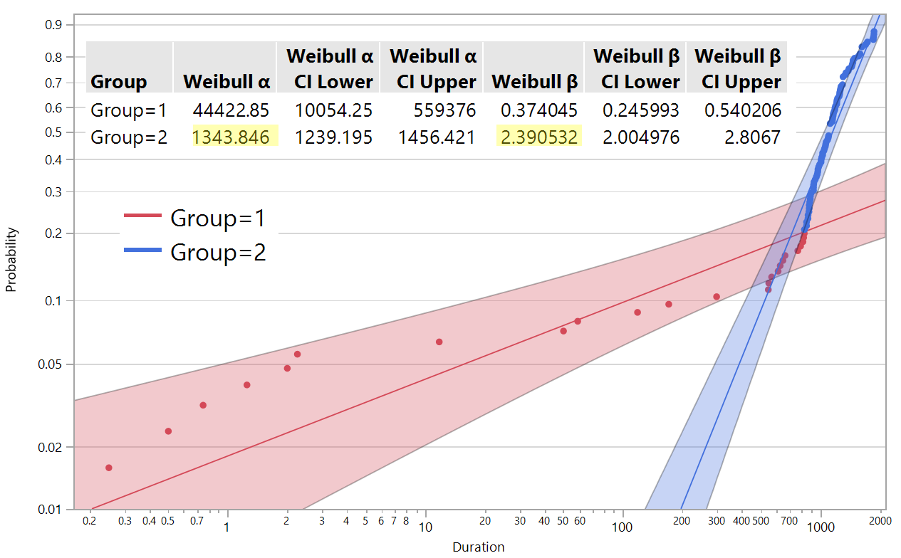
I made suggested changes to split reliability data to two failure modes, where split point is Portion 1 value from Competing Risk Mixture report.
The Weibull α and β distribution parameters of group 2 (see graph below) got same values as Weibull α and β distribution parameters from subset in my post above.
P.S.
Is there way to do Competing Risk Mixture in Fit Life by X platform?

- Mark as New
- Bookmark
- Subscribe
- Mute
- Subscribe to RSS Feed
- Get Direct Link
- Report Inappropriate Content
Re: distribution parameters mismatch between Competing Risk Mixture and SubSample in Life Data platform
What you did is not what I suggested. What you have done in the last using "Life Distribution - Compare Groups" is a third analysis in this thread of discussion. What you have done is technically identical to what you have done in your second analysis. That is why you get "same" results. I don't understand the objective, so I will stop trying to guide on your specific data. In the following, I will use JMP sample data sets to make my points, be useful in general to the audience who read this thread.
First, "Competing Risk Mixture" and "Competing Cause" are two different analyses. The terms "competing risk" and "competing cause" may be used interchangeably in the literature. They both take rows of observations, and each observation is a time-to-event observation. And each observation is associated with a cause. But in some experiments, you known the cause; in other experiments, you don't. When you don't have failure causes, you use Competing Risk Mixture. When you have failure causes, you use "Competing Cause". Competing Risk Mixture helps you to guess distributions of individual failure causes, but won't be able to tell the causes of individual observations for sure. Competing Cause fits distributions of individual failure causes, and failure cause is known information. Under normal use cases, there should not be confusion about which analysis to use, and one should not modify data in order to switch analysis types. "Appliance.jmp" is a sample data under Reliability sample data folder to illustrate Competing Cause. There is a Cause Code column in the table. The column "Y2" in "Mixture Demo.jmp", a sample data under Reliability sample data folder, is created to illustrate Competing Risk Mixture. There is no cause information in the table.
Second, when using Competing Cause, there is no need for user to modify data. The software modifies the data for the user to fit the model. Here is what the software does conceptually. I use "Appliance.jmp" as an example.
- For every cause code, create a copy of the entire data. Suppose the current cause code is 9. And I have a copy of entire data of 36 rows.
- Create two new columns: Left and Right.
- For every row, if the cause code is 9, simple copy over Time Cycles to both Left and Right. Row example, the second row.
- If cause code is not 9, copy Time Cycles to Left, but fill Right with a missing value. You may recognize this represents a right censored observation. Take the first row as an example, whose failure cause is 1. Because it is competing cause, cause 1 happened first. If we pretend 1 did not happen, and the system will fail due to cause 9, the failure time should be some where after 11 cycles, but we don't know when. So for this row, the software copies 11 to Left, and fill Right with a missing value.
- Now Left and Right are the new columns that should go to Y Time to Event role, if you want to fit a distribution to cause code 1.
This is what the new data look like:
If you analyze the modified data using Life Distribution like this:
You can get the same Weibull estimates same as those from Competing Cause analysis.
This is the result from Competing Cause by running the embedded script in Appliance.jmp.
And this is the result from Life Distribution using the modified data.
Repeat for all cause code values. And you get the full results of distributions for all causes. The software does all those for the user, and eventually aggregates all fitted distributions into one that is the failure distribution of the system.
To conclude, I want to emphasize, "Competing Risk Mixture" and "Competing Cause" are two different analyses. Decision of using which should be made upon whether there is information of failure causes.
In the end, to your last question, Fit Life by X does not support Competing Risk Mixture type distributions.
Recommended Articles
- © 2025 JMP Statistical Discovery LLC. All Rights Reserved.
- Terms of Use
- Privacy Statement
- Contact Us