- New to JMP? Let the Data Analysis Director guide you through selecting an analysis task, an analysis goal, and a data type. Available now in the JMP Marketplace!
- See how to install JMP Marketplace extensions to customize and enhance JMP.
- Subscribe to RSS Feed
- Mark Topic as New
- Mark Topic as Read
- Float this Topic for Current User
- Bookmark
- Subscribe
- Mute
- Printer Friendly Page
Discussions
Solve problems, and share tips and tricks with other JMP users.- JMP User Community
- :
- Discussions
- :
- Reference test and formula associated with the graph
- Mark as New
- Bookmark
- Subscribe
- Mute
- Subscribe to RSS Feed
- Get Direct Link
- Report Inappropriate Content
Reference test and formula associated with the graph
Dear All,
I am new to using JMP software,
I created this topic concerning the graphs generated by the JMP software,
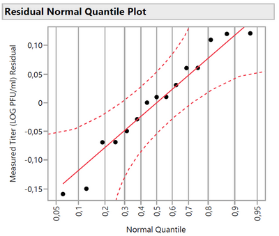
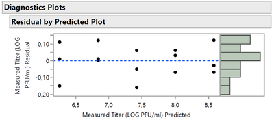
As you can see in the attachment, I have generated the "Residual by Predicted Plot" and also the "Residual Normal Quantile Plot" graphs. This corresponds perfectly to my needs, but for my knowledge, I'd like to know what statistical test was carried out to obtain the graphs, as well as the associated formulas, if any?
Could you help me with this, please?
Thank you for your time,
Best regards,
Accepted Solutions
- Mark as New
- Bookmark
- Subscribe
- Mute
- Subscribe to RSS Feed
- Get Direct Link
- Report Inappropriate Content
Re: Reference test and formula associated with the graph
The residual plots are part of the post-analysis to assess model adequacy and the assumptions of the regression model. The residual is the predicted or fitted Y minus the observed Y. The residual estimates the statistical error.
The assumptions include that the statistical errors are independent and identically normally distributed with a mean of zero and a constant variance (i.e., variance is independent of Y). The normal quantile plot results from fitting a normal distribution and plotting the fitted quantiles against the residual value. The scaling is unique to each distribution model. The scaling results in a linear relationship between the quantiles and the errors. In the case of the normal quantile plot, the slope of the line is the standard deviation, and the y-intercept is the mean. If you see a pattern that is not linear overall, then the assumption of normal errors is violated. If you see a linear pattern but one or more quantiles are far from the line at the ends of the plot, then you might have outliers.
The residual by predicted plot is used to assess the adequacy of the model. The identity reference line shows where Y = X. You expect the observations to follow this line. A large departure from the line overall suggests lack of fit. A large departure from the line by some observations suggests outliers. This plot also helps assess the constant variance. The plot should exhibit a uniform spread of residuals from low to high predicted values. That is, the magnitude of the residuals does not depend on the response. The appearance of a funnel shape indicates a violation of this assumption. Ordinary least square regression is inappropriate in such cases.
The assumption that all the statistical error is in Y and none of it is in X is not assessed with the residual plots. They also assume the same thing.
- Mark as New
- Bookmark
- Subscribe
- Mute
- Subscribe to RSS Feed
- Get Direct Link
- Report Inappropriate Content
Re: Reference test and formula associated with the graph
Did you read the documentation about the Bivariate platform?
- Mark as New
- Bookmark
- Subscribe
- Mute
- Subscribe to RSS Feed
- Get Direct Link
- Report Inappropriate Content
Re: Reference test and formula associated with the graph
Dear Mark,
Thanks for your answer,
Indeed, I find the following formula:
If I understand correctly, this means that JMP generates different graphs (see below) from this formula, is that correct?
Thank you for your help,
Best regards,
- Mark as New
- Bookmark
- Subscribe
- Mute
- Subscribe to RSS Feed
- Get Direct Link
- Report Inappropriate Content
Re: Reference test and formula associated with the graph
The residual plots are part of the post-analysis to assess model adequacy and the assumptions of the regression model. The residual is the predicted or fitted Y minus the observed Y. The residual estimates the statistical error.
The assumptions include that the statistical errors are independent and identically normally distributed with a mean of zero and a constant variance (i.e., variance is independent of Y). The normal quantile plot results from fitting a normal distribution and plotting the fitted quantiles against the residual value. The scaling is unique to each distribution model. The scaling results in a linear relationship between the quantiles and the errors. In the case of the normal quantile plot, the slope of the line is the standard deviation, and the y-intercept is the mean. If you see a pattern that is not linear overall, then the assumption of normal errors is violated. If you see a linear pattern but one or more quantiles are far from the line at the ends of the plot, then you might have outliers.
The residual by predicted plot is used to assess the adequacy of the model. The identity reference line shows where Y = X. You expect the observations to follow this line. A large departure from the line overall suggests lack of fit. A large departure from the line by some observations suggests outliers. This plot also helps assess the constant variance. The plot should exhibit a uniform spread of residuals from low to high predicted values. That is, the magnitude of the residuals does not depend on the response. The appearance of a funnel shape indicates a violation of this assumption. Ordinary least square regression is inappropriate in such cases.
The assumption that all the statistical error is in Y and none of it is in X is not assessed with the residual plots. They also assume the same thing.
Recommended Articles
- © 2026 JMP Statistical Discovery LLC. All Rights Reserved.
- Terms of Use
- Privacy Statement
- Contact Us


